“Technical
Procedures Bulletin” for the T382 Global Forecast System
(final revision October 26, 2005)
EMC: Jordan Alpert, George Gayno, Mark Iredell, Robert
Kistler, Sarah Lu,
Jesse Meng, Kenneth Mitchell, Shrinivas Moorthi,
Suranjana Saha, Joseph Sela,
Russ Treadon, Helin Wei, Glenn White, Xingren Wu, Michael
Young, Yuejian Zhu
NCEP Centers: Arun Kumar, CPC, Craig Long, CPC, Peter Manousos, HPC, David Michaud, NCO, Richard Pasch, TPC, Jae Schemm, CPC, Joseph Sienkiewicz, OPC, Steven Silberberg, AWC, Steven Weiss, SPC
INTRODUCTION
NCEP implemented major changes to its Global Forecast System (GFS) on May 31,
2005. The horizontal resolution
increased from approximately 50 km (T254) to approximately 35km (T382) in both
the analysis and forecast model for the four GFS cycles at 00, 06, 12, and 18
UTC. The vertical resolution, which had varied from 64 to 28 layers, is now 64 layers for the
entire 16-day forecast. Changes to the
analysis consist of additional radiance data, enhanced quality control, and
improved emissivity calculations over snow and ice. Changes to the model consist of new sea-ice and land-surface
models, modified vertical diffusion, and enhanced mountain blocking.
In conjunction with the model changes, additional GFS products are now stored in the NCEP ‘master file’ system, which is accessible to NCEP scientists. The structure of the model has been reworked to be computationally more efficient and to be ready in the future for ESMF (Earth System Modeling Framework) and a hybrid (sigma, p) vertical coordinate. In addition, minor upgrades were made on June 14 to the land-surface model, and on July 7 to the upper stratosphere analysis, in order to address issues noted during the evaluation phase. More details regarding these topics are shown in the sections below. Please note that a variety of labels are used to differentiate the new GFS from the old GFS in the figures, e.g. pry, prx, prz, GFSX, GFSp …
The new GFS uses the 35km (T382) horizontal resolution out to 180 hours and 70km (T190) out to 384 hours. The 64-layer vertical resolution is the same for the entire forecast. Comparison of the new and old GFS is shown below, with the necessary telescoping of resolution for computational efficiency:
New: T382L64, 0-180 hours; T190L64, 180-384 hours.
Old: T254L64, 0-84 hours; T170L42, 84-180 hours; T126L28, 180-384 hours.
1. The amount of assimilated radiance data increases substantially with the addition of AQUA AIRS and AQUA AMSU-A data. The intelligent thinning algorithm, used when reading the radiance data, has been modified to allow for grouping of data based on sensor type, in order to spread data use more evenly over the globe. Relative weighting among the different data sources within each group is permitted, thereby allowing one to choose data that may have a better chance of passing quality control checks. For example, assume data-types X and Y are assigned to the same infrared group, but X data are given a threefold greater relative weighting. If a thinning box contains both X and Y data, the X data-type will have more influence, assuming additional quality control decisions are comparable for the two types of data.
2. The quality control of infrared radiances is enhanced by the addition of a new cloudiness algorithm, where estimates of percent cloudiness are obtained using observed and simulated IR brightness temperatures as well as brightness temperature sensitivities computed from the CRTM (Community Radiative Transfer Model, formerly known as OPTRAN). An estimate is also made of the cloud-top pressure. This information is then used in subsequent quality control decisions to allow use of data down to the cloud-contaminated level.
3. A new microwave emissivity model over snow and ice is added. This model was developed by scientists within NESDIS/ORA and implemented by Okamoto and Derber (2005), and it allows an increase in the use of microwave data over snow and ice-covered surfaces during the global analysis.
1. The new sea-ice model is based on Winton’s (2000) three-layer (two equally thick sea-ice layers and one snow layer) thermodynamic process. It predicts sea-ice/snow thickness, surface temperature, and ice temperature structure. The analyzed fractional ice cover is kept unchanged for the entire forecast, but there is an option to use climatology for daily sea-ice concentration. The old scheme simply used a fixed sea-ice array, either 100% or 0% ice cover. For the new model, heat and moisture fluxes and albedo are treated separately for ice and open water in each grid box (Wu et al. 1997).
2. The GFS land-surface model component was substantially upgraded from the Oregon State University (OSU) land surface model to EMC's new Noah Land Surface Model (Noah LSM). The Noah LSM (Chen, et al. 1996; especially sections 3.1.1 and 3.1.2, Koren et al. 1999, and Ek et al. 2003) represents about 10 years of substantial upgrades over its OSU ancestor model of the mid 1990's. These upgrades were developed and tested by the EMC Land Team, assisted by its many collaborators, including NWS/OHD, NCAR/RAP, NESDIS/ORA, AFWA, NASA/GSFC/HSB, and several PIs of the GEWEX Americas Prediction Project (GAPP), which is sponsored by the NOAA Office of Global Programs (OGP). This new Noah LSM is also operational in NCEP's regional, mesoscale models. Details of the Noah LSM are presented in the Appendix. In summary the new land-surface parameterization has 4 sub-surface layers, rather than the two layers used in the OSU scheme. It also contains improved treatment of frozen soil, ground heat flux, and energy/water balance at the surface, along with reformulated infiltration and runoff functions and an upgraded vegetation fraction.
To obtain initial values of soil moisture and soil temperature, the Noah LSM cycles continuously on itself in the GDAS cycles. Values are updated every model time step in response to forecasted land-surface forcing (precipitation, surface solar radiation, and near-surface parameters: temperature, humidity, and wind speed). Since the land component of the GDAS is forced by GFS model precipitation, rather than observations, it is constrained by nudging soil moisture, with a 60-day relaxation, towards an externally supplied global soil moisture monthly climatology.
The old GFS suffered from overly rapid snow-pack depletion in winter (from both too much snowmelt and snow sublimation). A series of 29 one-day forecasts in December 2004 indicates that the new GFS, with the Noah LSM, substantially reduces the tendency for early snow-pack depletion. The 24hr forecast snow cover over N. America is compared with the snow analysis for 2 cases (Fig 1, Fig 2). The upper and lower plots show the new GFS and the old GFS, respectively, while the blue/green and red/orange colors display areas where the GFS under-forecasts and over-forecasts snow cover.
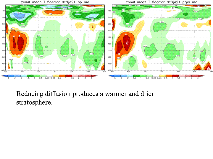
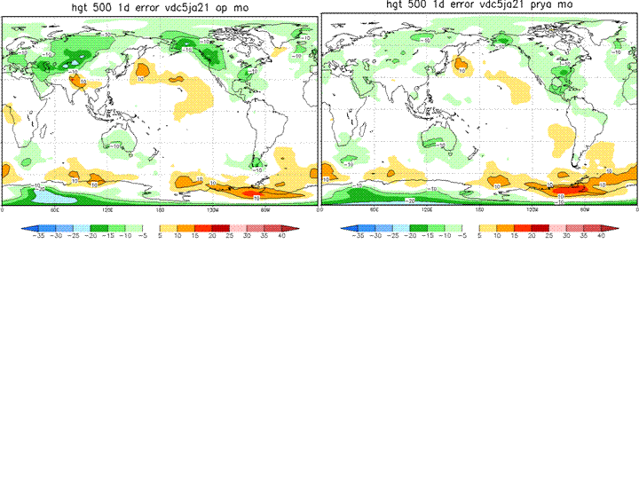
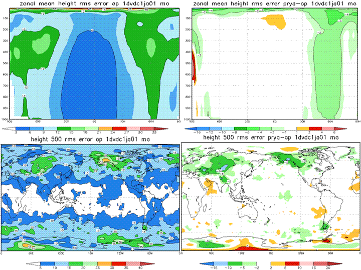
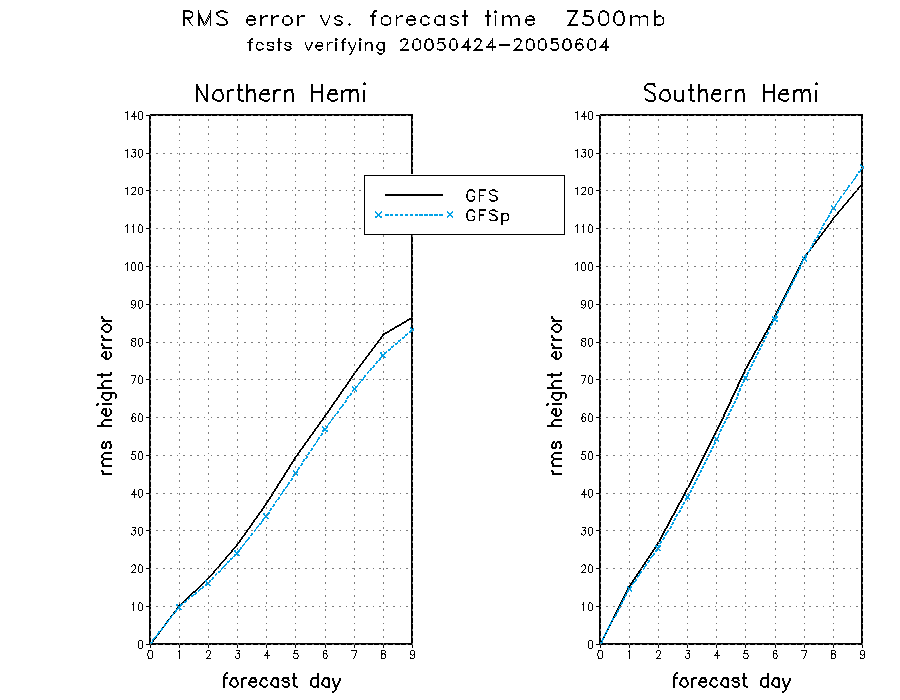
3. Changes are made to the parameterizations of mountain blocking and vertical diffusion. It was determined from a series of 1-day experiments that enhancing the orographic height by 10% of the mountain variance, reminiscent of ‘enhanced orography’ applied in old versions of the model, during the calculation of the mountain blocking dissipative forces, improved results. Similarly, it was found that reducing both the background diffusion in the free atmosphere and the turbulent diffusion length scale from 150 meters to 30 meters in stable cases improved the results. During winter 2004-2005, the combined changes to mountain blocking and reduced vertical diffusion produced improved (warmer and drier) zonal mean stratospheric temperature at day 5 (Fig 3), as well as lower mean 500 hPa height errors at day 1 for December 5, 2004-January 21, 2005 (Fig 4). Improvements in new GFS one-day RMS height errors for December 1, 2004-January 1, 2005 can also be seen in Fig 5, where the error differences (new GFS minus old GFS) are shown on the right and the RMSE for the old GFS on the left. Since mean orography is retained, there are fewer problems assimilating surface observations in the analysis.
1. Soil moisture and temperature: The old second soil layer (10-200 cm below ground surface) is replaced with 3 soil layers (10-40 cm, 40-100 cm, and 100-200 cm). The first soil layer (0-10 cm) is unchanged, yielding a total of four (rather than two) soil layers in the new GFS.
2. Potential Vorticity Unit (PVU) surfaces: In the old GFS, geopotential height, temperature, pressure, vertical windshear, and u/v winds on the +2000 and –2000 PVU surfaces were labeled incorrectly as 2 PVU surfaces. This has been corrected in the new GFS.
1. Add upper stratospheric data at 7, 5, 3, 2, and 1 hPa.
2. Accommodate new model physics by adding 15 records: clear and all-sky UV-B downward SW radiative flux, soil moisture and temperature for deep soil layers (10-40 cm, 40-100 cm, 100-200 cm), liquid soil moisture (4 soil layers), plant-canopy surface water, sea-ice thickness, and physical snow depth. By retaining the traditional water-equivalent snow depth, the density of the snow-pack can be obtained from the ratio of water-equivalent to physical snow depths.
3. Potential Vorticity Unit (PVU) surfaces: Added 6 PVU surfaces (for a total of 8 at
500, 1000, 1500, 2000, -500, -1000, -1500, -2000) and corrected units (see above); with each PVU surface containing 6 records (geopotential height, temperature, pressure, vertical wind shear, u-wind, v-wind).
4. Maximum wind level: new GFS searches pressure levels 500-100 hPa, rather than 500-70 hPa.
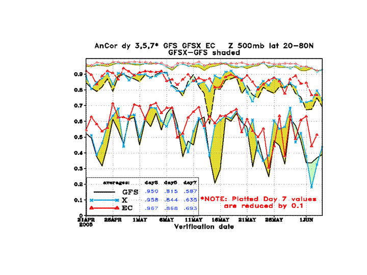
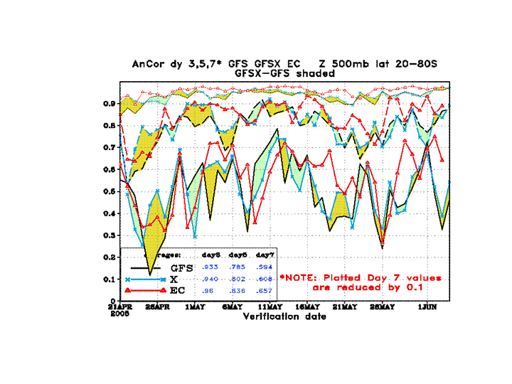
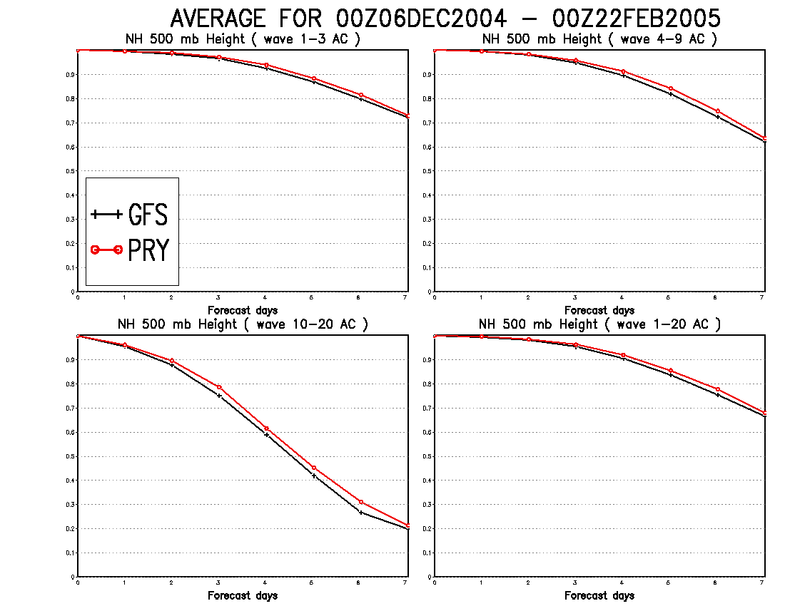
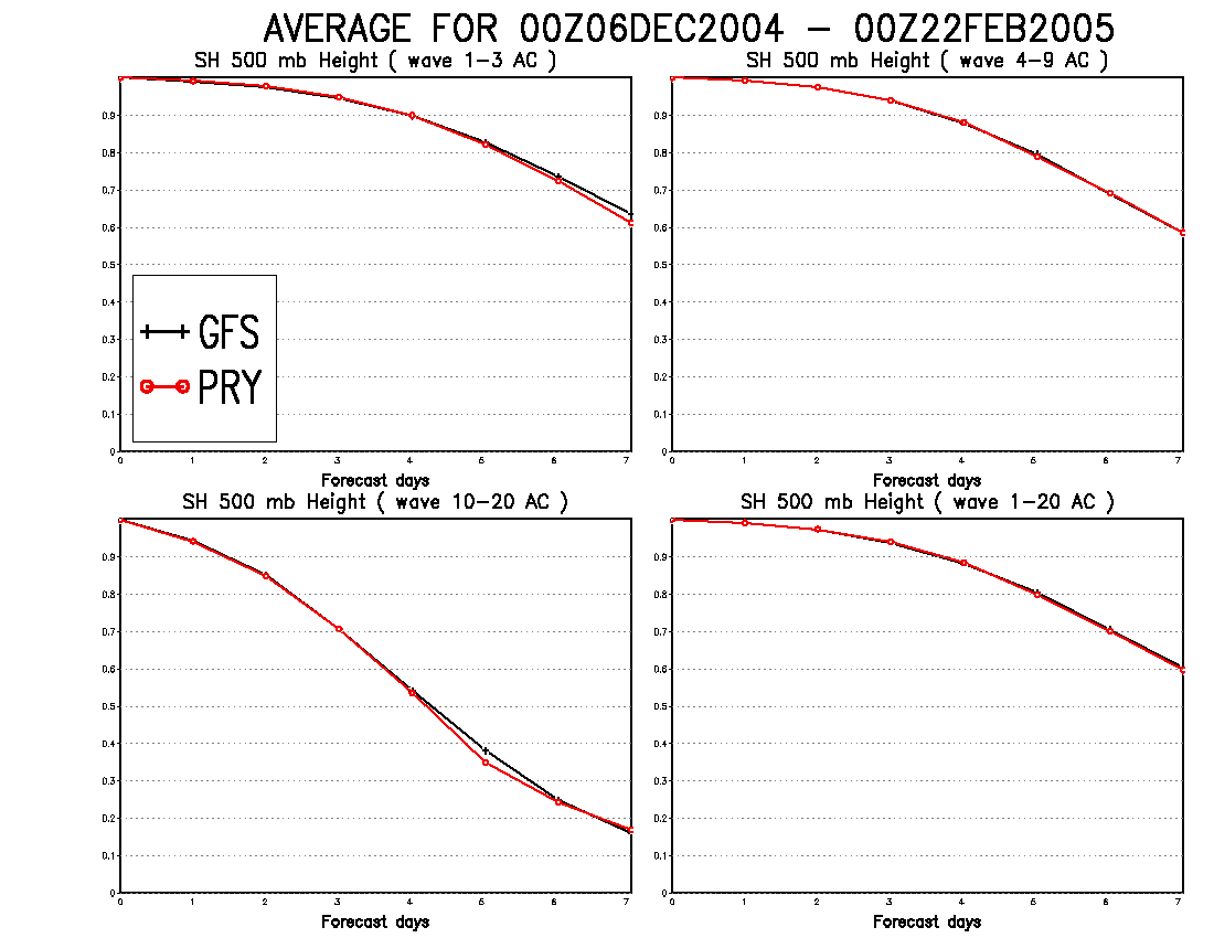
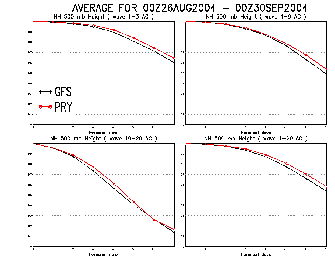
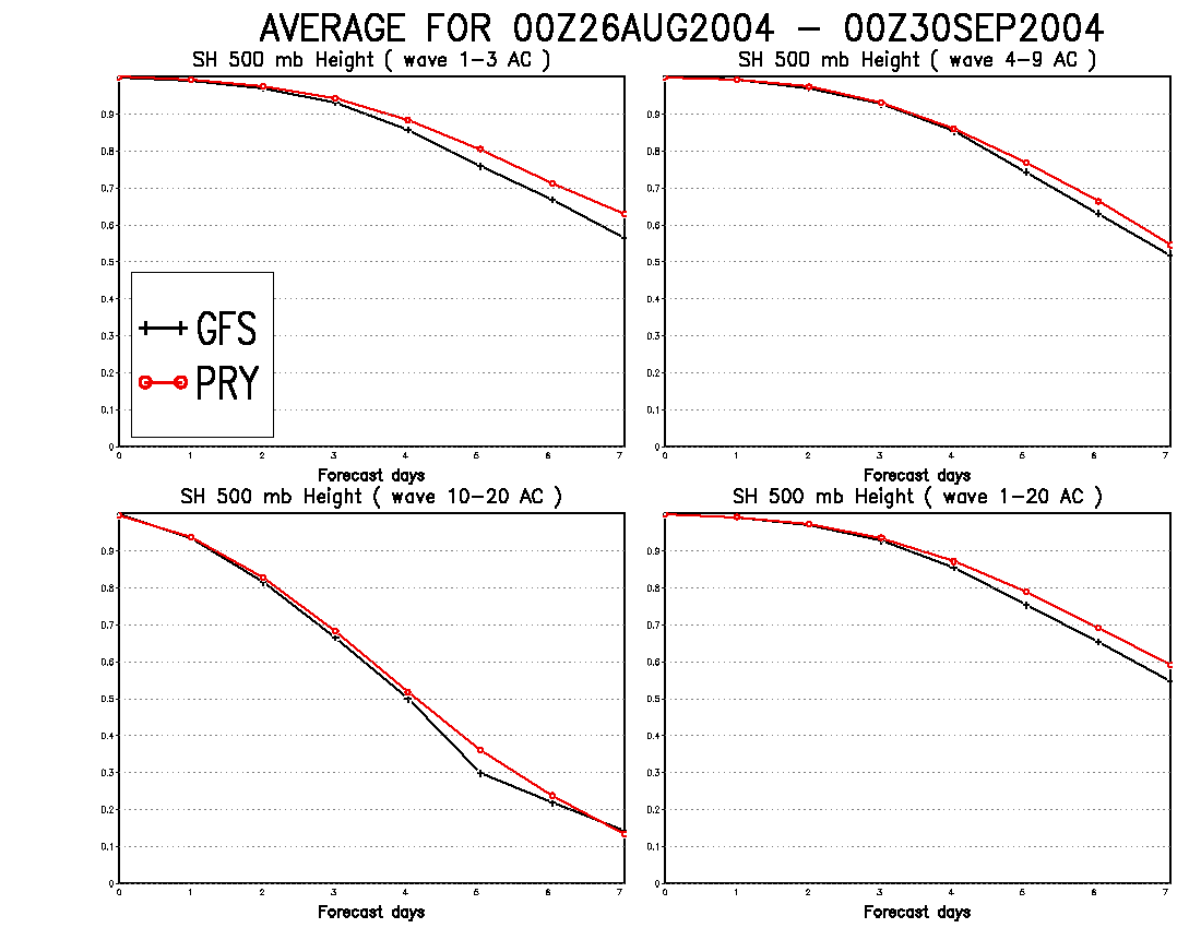
All NCEP Centers participated in the evaluation of real-time parallel forecasts in April and May 2005, and of retrospective forecasts made using both Aug-Sep 2004 and Dec-Feb 2004/2005 data. Verifications against analyses of the new GFS show general improvements in a number of forecast products. Comparison of Northern Hemisphere (NH) and Southern Hemisphere (SH) 500 hPa geopotential height anomaly correlation (AC), for forecast days 3, 5, 7, verifying April 21-June 3, shows a consistent forecast improvement for the new GFS in the NH (‘yellow’ shading in Fig 6, Fig 7) and mixed results in the SH. For the retrospective tests, the 500-hPa AC die-off curves (Fig 8, Fig 9, Fig 10, Fig 11) show that the new GFS clearly improves the scores through all wave-number groups, except in the case of the Dec-Feb Southern Hemisphere results, where the models were comparable. The daily scores for day 5 forecasts (not shown) indicated reasonable day-to-day consistency in these results.
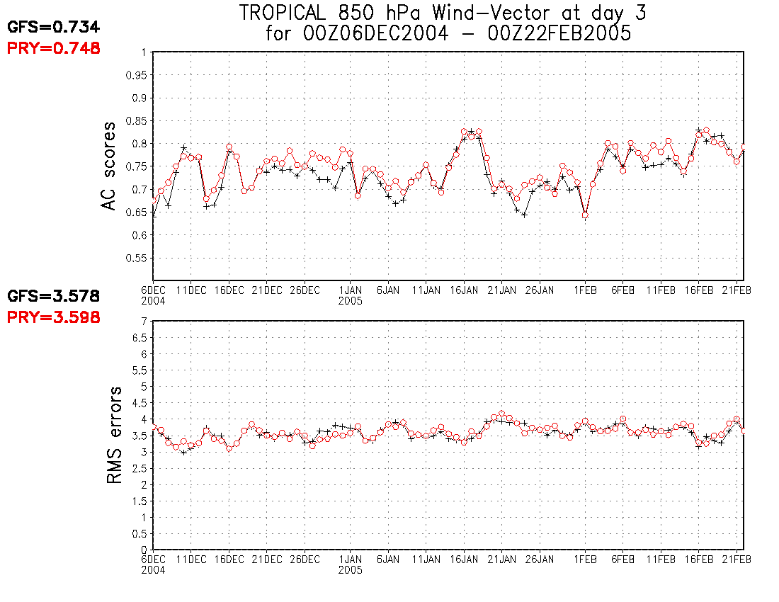
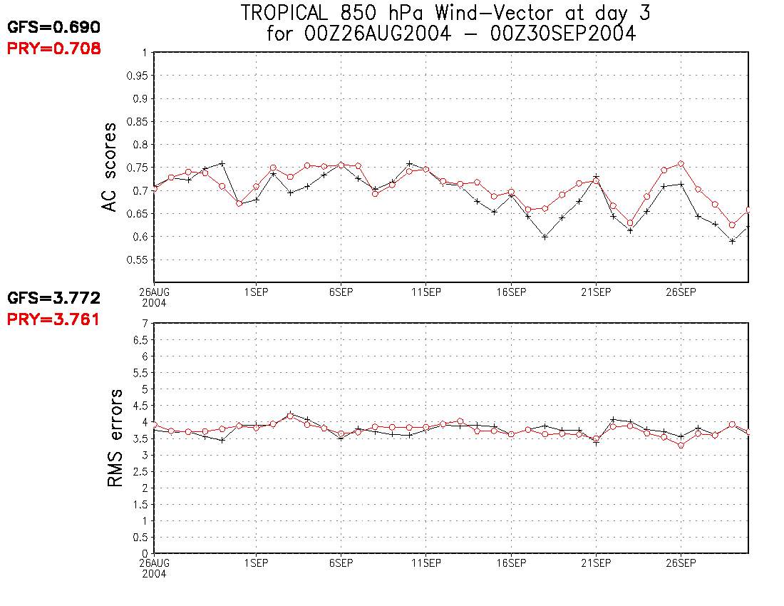
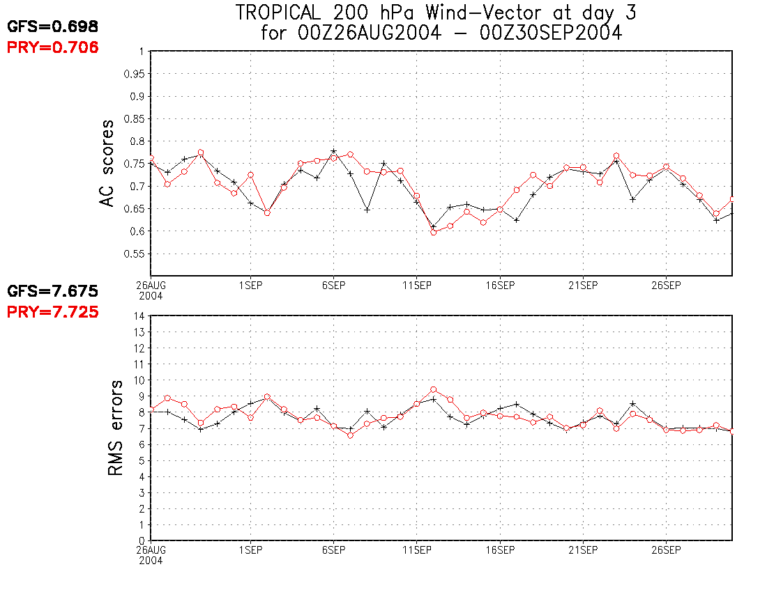
Comparison of the retrospective tropical wind AC and RMS error scores at 850 hPa and 200 hPa, show slightly better AC and slightly worse RMS errors for the new GFS (Fig 12, Fig 13, Fig 14, Fig 15).
New GFS precipitation skill scores show a clear improvement in the winter (Fig 16, Fig 17, Fig 18), except for amounts greater than 50 mm/24hrs, where there are very few cases. Real-time scores in April 2005 show new GFS improvement after the first 36 hours of the forecast (Fig 19). However, precipitation skill scores for the summer cases were somewhat worse in the initial pre-implementation testing of the new GFS (Fig 20, Fig 21, Fig 22). Upon further investigation, the lower summer precipitation forecast skill in the new GFS was attributed to its larger positive precipitation bias, which, in turn, was attributed to a larger positive bias in summer surface evaporation in the Noah LSM over regions of non-sparse vegetation cover (e.g. eastern CONUS). Further pre-implementation testing culminated in modifications to the canopy resistance parameters in the land-surface scheme, which yielded (1) lower surface evaporation than in the old GFS over most vegetation classes and (2) a decrease in the positive precipitation bias of the old GFS. These changes were implemented operationally on 14 June 2005 and the improved summer precipitation skill scores are discussed below (see paragraph 2 in the "issues addressed" section).
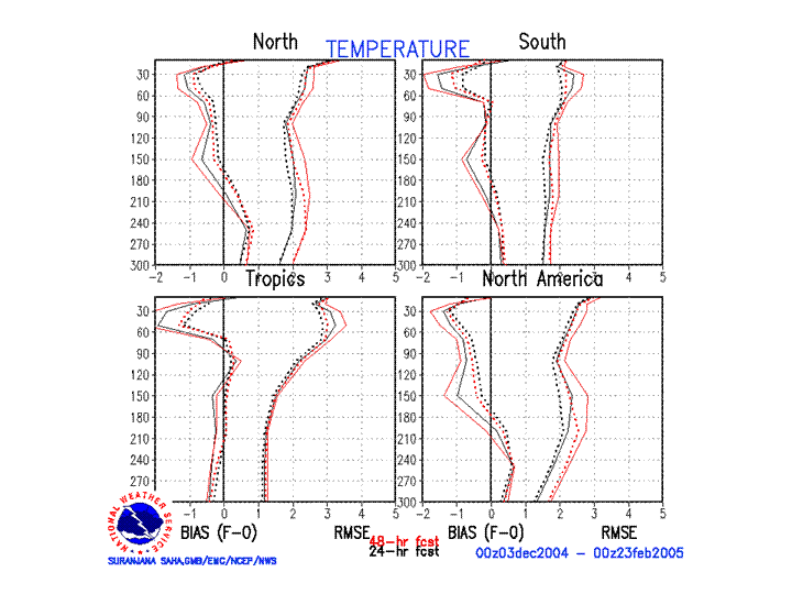
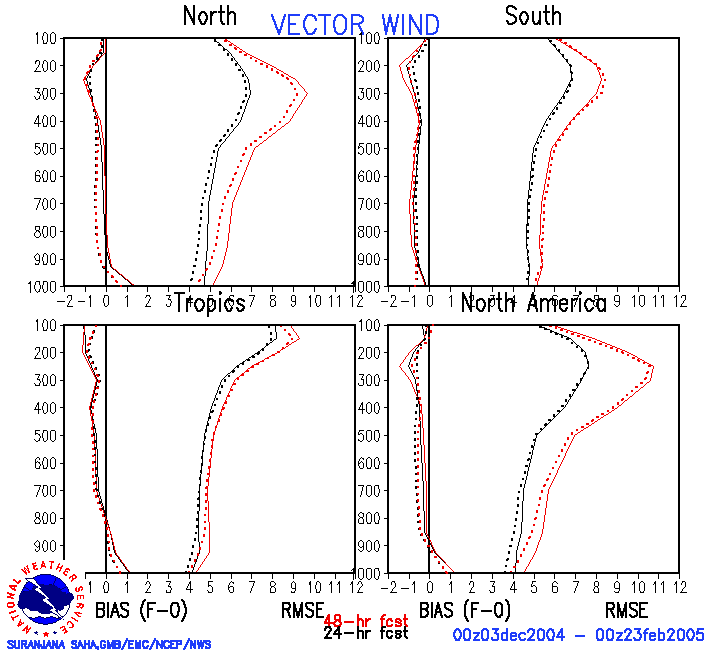
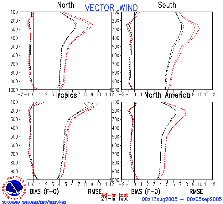
Verifications against observations were made for the old and new GFS during the retrospective time periods 28 Jul – 21 Aug 2004 and 3 Dec 2004 – 23 Feb 2005. In the graphics for this section, the new model is shown by dotted lines and labeled as “pry”; the old model by solid lines and labeled “fnl”. The vertical profiles show two groups of lines for each region (NH, SH, tropics and N America). The group of profiles on the left depicts bias; the group on the right, rms error. For stratospheric temperature forecasts at 24 and 48 hours, the new model showed improvement in all regions and at almost all levels from 300 through 30 hPa during both time periods (Fig 23 and Fig 24). For the tropospheric temperatures, the results (Dec-Feb period only, Fig 25) were mixed, with rms errors better in the NH and about even in the SH. Scores were marginally worse in the tropics, SH and Asia. Negative biases in the lower tropical troposphere were worse in the new model.
Vertical profiles of wind speed bias and rms vector errors at 24 and 48h for the Dec-Feb period are shown in Fig 26 and for the Aug-Sep period in Fig 27. For Dec-Feb, the new model was clearly superior in the NH and somewhat better in the tropics; for Aug-Sep, the new model is slightly worse, but the period of averaging was only 24 days.
It should be noted that the verifications against analyses for this period indicated only that the models were comparable. There was an underestimate of the Asian 200-hPa jet in both models.
SUBJECTIVE EVALUATION from the NCEP Centers
OPC
The new model’s 500 hPa
Anomaly Correlation scores in NH winter show considerable improvement over the
T254 model for all wave numbers. In
particular, improvement is significant for cyclone scale at days 3 and 4. The old GFS usually forecasts multiple weak
cyclones in developing oceanic storm situations, thereby producing a
weaker-than-observed wind warning. The
new GFS shows a more consolidated storm, thus providing better guidance to OPC
forecasters (Fig 28).
HPC
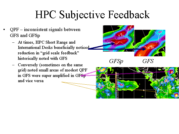
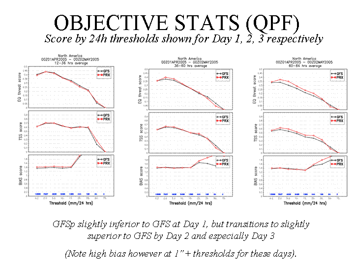
Short range (0-84 hours), medium range (out to day 8), and international desk forecasters agree that the new GFS is offering a better mass field solution (Fig 29), but the medium range forecasters find that the new model offers less run-to-run continuity. HPC forecasters have been unable to reach a conclusion on QPF (Quantitative Precipitation Forecast) performance. Objective evaluation shows the new GFS slightly inferior at day 1, but superior at days 2 and 3. The international desk is concerned about excessive rainfall amounts in the tropics. (Fig 30, Fig 31). However, HPC will support the implementation, since EMC is actively working to make a QPF improvement in June 2005 (see issue #2 below).
CPC
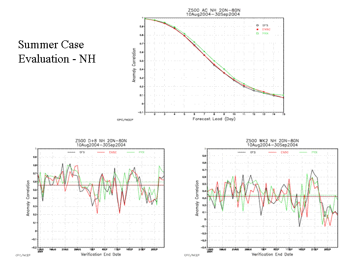
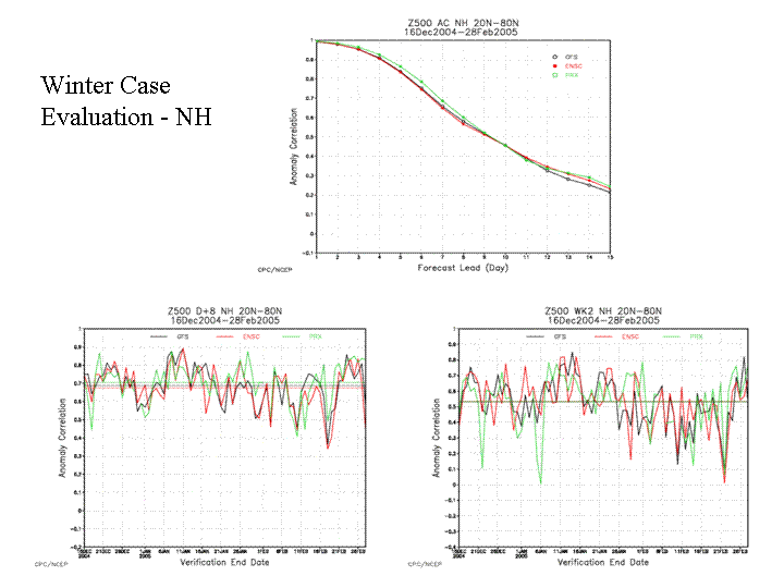
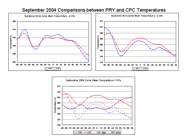
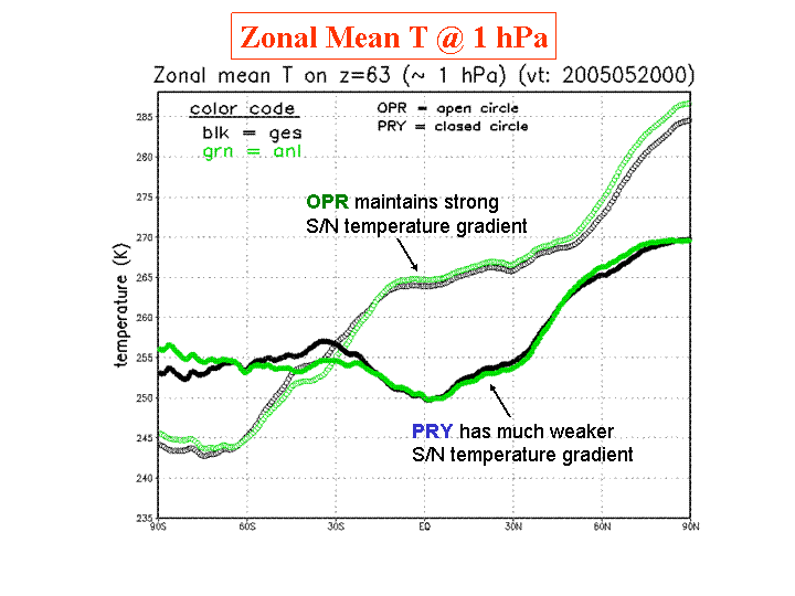
In both summer (10 August-30 September, 2004) and winter (16 December 2004-28 February 2005), forecast skill of the new GFS in the Northern Hemisphere is improved up to day 10, but not in the week 2 forecasts (Fig 32, Fig 33). This is visible especially in the D+8 summer forecasts. The upper stratosphere (above 10 hPa) is significantly colder in the new GFS. Comparison of the old and new GFS analyzed zonal mean temperatures, with CPC’s analysis, shows general agreement below 10 hPa, but the new GFS is 5-10 degrees colder above. Available lidar data show the CPC analysis to have zero bias at 2 hPa, and a 3-5 degree warm bias at 1 hPa. At 5 and 2 hPa, all zonal means mirror each other, but at 1 hPa the new GFS zonal means are very inconsistent with the underlying 2 hPa data. (Fig 34).
TPC
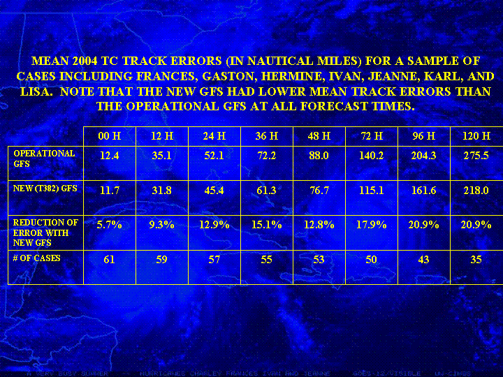
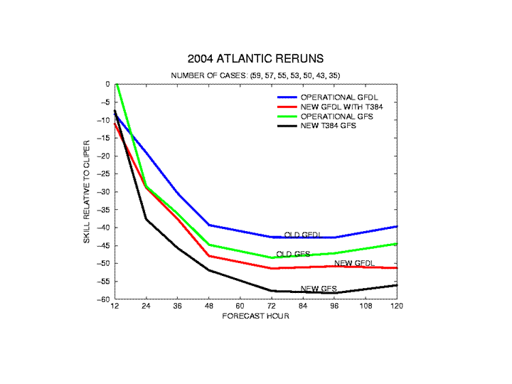
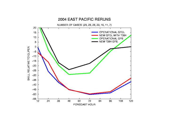
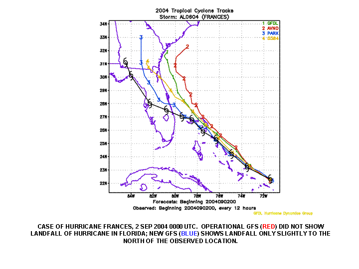
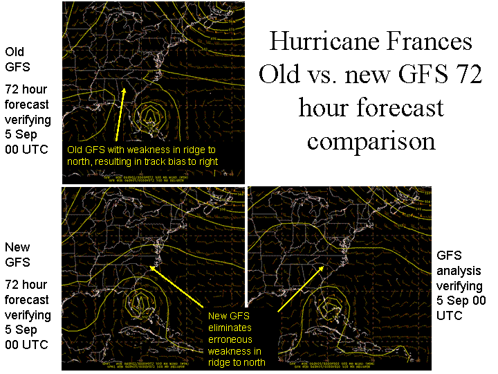
Results of the retrospective runs from the 2004 hurricane season show the new GFS having a significant reduction in Atlantic tropical cyclone track forecast errors for these cases (Fig 35, Fig 36), while showing little change in the East Pacific (Fig 37), where the old GFS had little skill. The forecasts of landfall for Frances (Fig 38, Fig 39) and Jeanne were improved in the new GFS. Although there is on average no significant difference in the skill of forecasts of other tropical weather features, TPC does note an example of an improved baroclinic low forecast from 1 May 2005 over Florida.
AWC
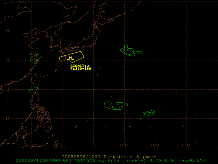
Jet stream guidance is improved in the new GFS, with wind maxima 5-10 m/s stronger. Additionally the new GFS has much, much improved turbulence guidance. Vertical wind shear in the new GFS is much stronger than the old GFS. In a recent case, off the East Asian coast, the Richardson number (Ri) diagnostics in the new GFS show values of Ri < 0.5 where severe turbulence was observed (the yellow SIGMET on Fig 40), while the old GFS Ri's were generally not below 1 (Fig 41). Although there is not a turbulence-reporting network to provide verification over large regions, the ability of the new GFS to place Ri values of less than 1 near coincident pilot reports of turbulence is considered a significant step forward.
SPC
Evaluation of the new GFS has been made using the parallel system during April and May 2005. In general, the new GFS is as good as or better than the old system, and it is anticipated that there may be small improvements to experimental medium range outlooks. Moisture and instability forecasts are often similar, but where there are differences, the new GFS forecasts of 2-meter dew points and CAPE tend to be larger (an improvement). Increased horizontal resolution in the new GFS appears to improve temperature and moisture patterns, as well as to strengthen and better define low and mid-level jet streaks. Also, the new GFS had better specification of return-flow moisture axes, which are precursors to some spring severe weather episodes. Finally, there appeared to be evidence that the new GFS had more meaningful details evident along boundaries such as dry lines and warm fronts.
NCO
NCO/EMC collaborative efforts with machine resources (devhigh) allowed a 20-day-earlier implementation date. There were 150 days of retrospective runs made on the ‘white’ machine, at about 5 forecast days each day. If EMC had only used the ‘blue’ machine, it would have been slower, advancing 3 forecast days each day! The software changes in the parallel GFS ran without failure and did not delay product delivery times. Changes in product format and volume were coordinated to fit within storage resources. The increase in computational resources of the new GFS fit within the projected ‘production window’.
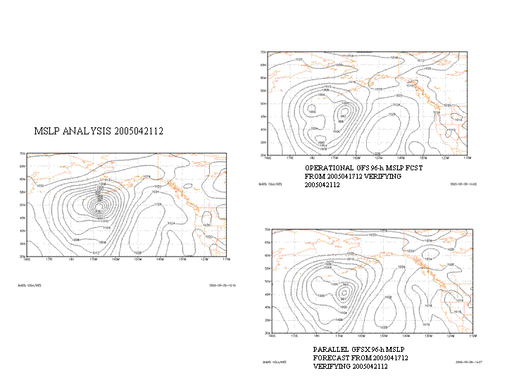
1. Stratospheric temperature at 1 hPa: New GFS temperature analyses above 5 hPa have not been very good since the May 31 implementation (Fig 42). The SSI component of the GFS could not properly handle over one hundred channels of AIRS data until sub-layers were added in the two topmost model layers. This correction was implemented in early July 2005. Temperature fields at 7, 5, 3, 2 hPa are now of acceptable quality, while 1-hPa temperatures in polar regions were improving on a daily basis (Fig 43). However, the 1-hPa tropical data differed from the CPC analyses by 5 - 10 degrees and it was anticipated that they would take several more weeks to settle into agreement with them.
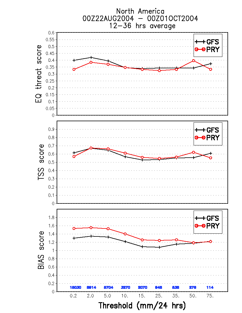
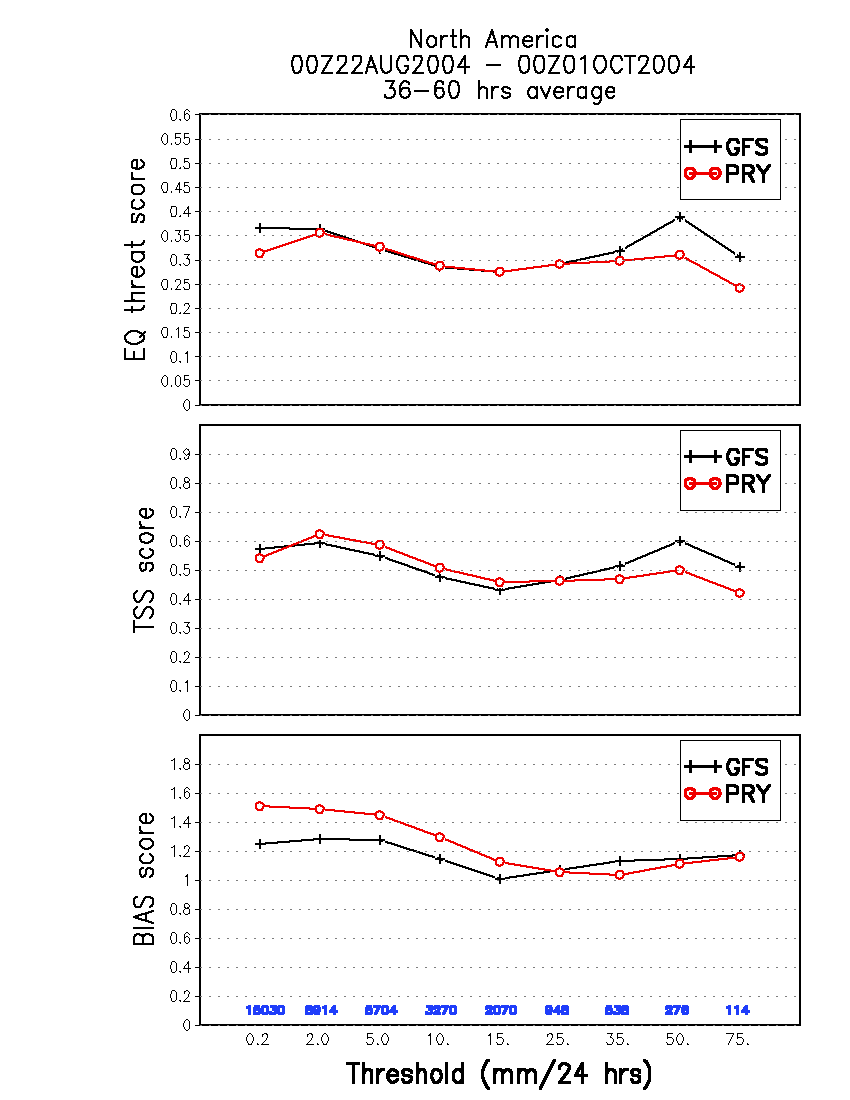
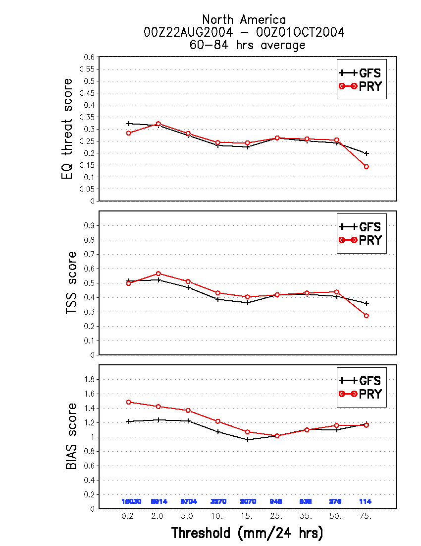
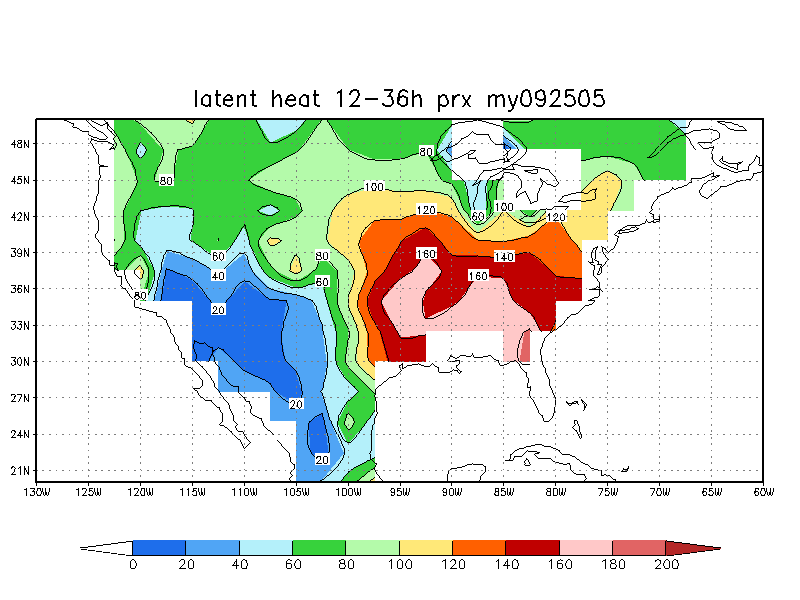
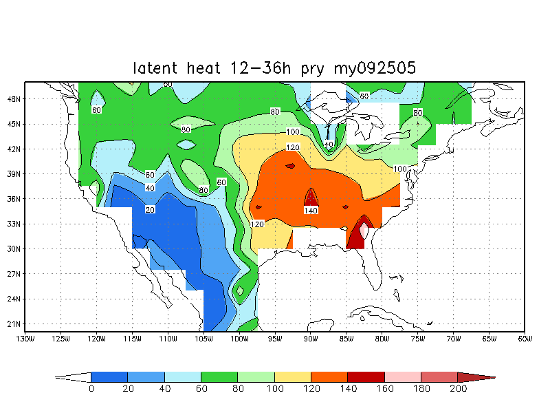
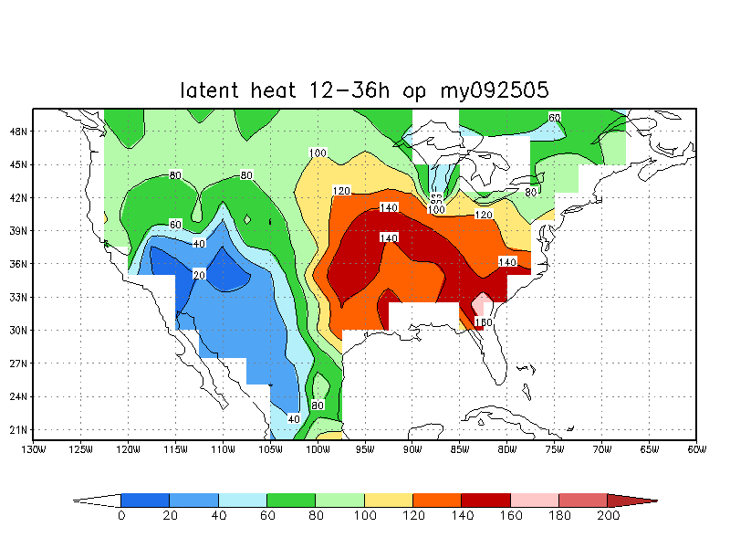
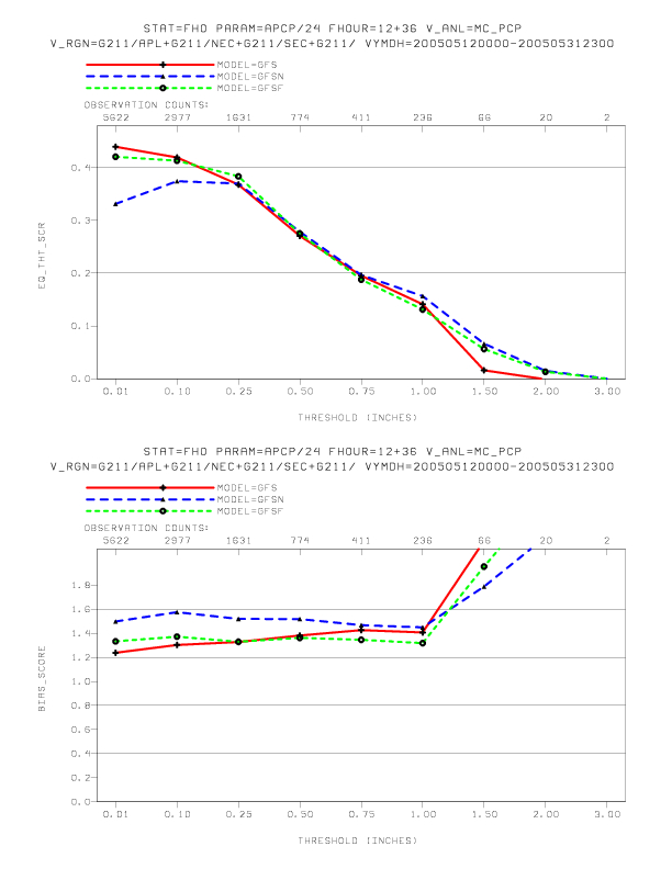
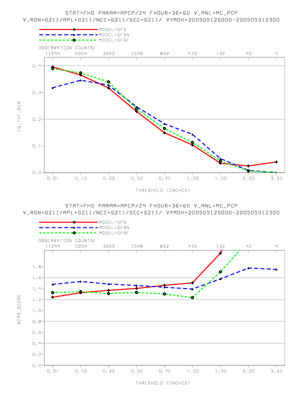
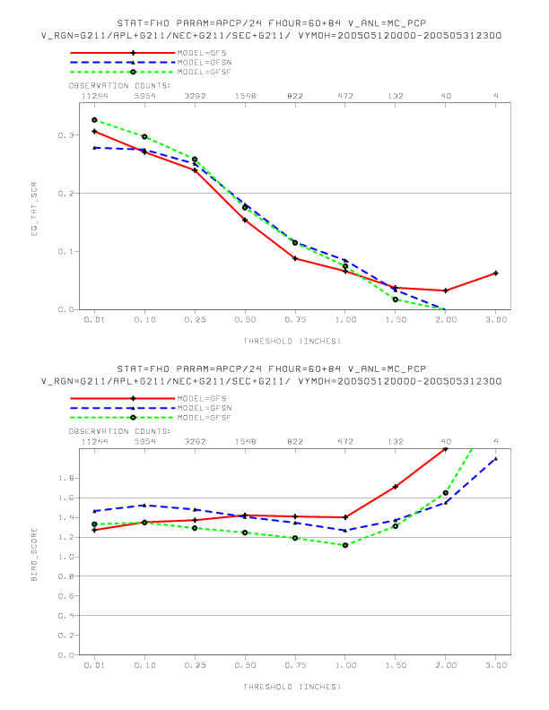
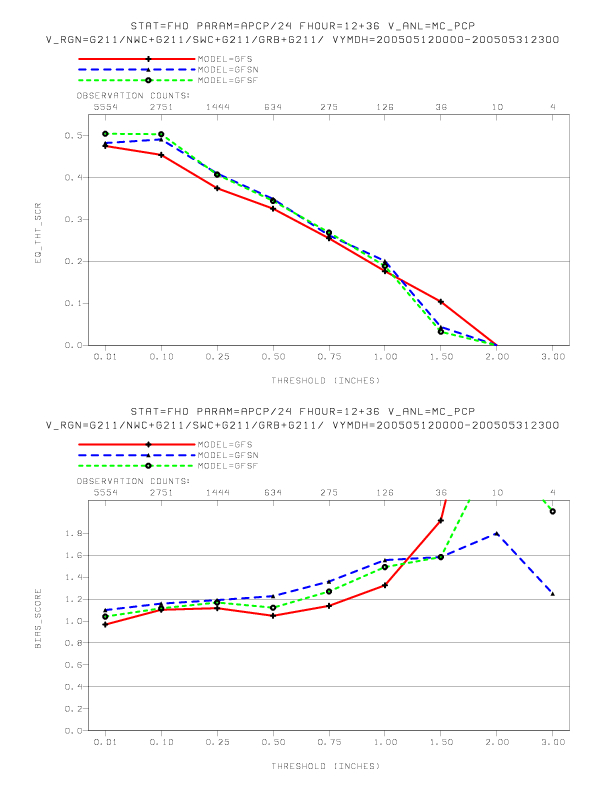
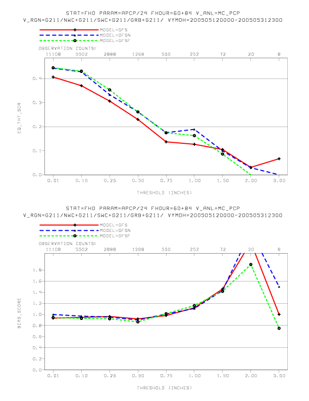
2. Cool moist bias in model lower layers: A modification was implemented on 14 June 2005 to the land model in order to increase canopy resistance by tuning two parameters (including the minimal stomatal resistance) in the Noah LSM formulation. In parallel tests during May 2005, the increased canopy resistance reduced the surface evaporation over non-arid land regions, during seasons of non-sparse green vegetation - compare the average daily surface latent heat flux (W/m2) during 9-25 May for the new GFS, both before (Fig 44b) and after the canopy resistance change (Fig 44c), and the old GFS (Fig 44a). The reduced surface evaporation, in turn, alleviated the near-surface cool and moist bias and reduced the excess precipitation amounts; results are shown for East CONUS stations at 12-36 hours (Fig 45a), 36-60 hours (Fig 45b), and 60-84 hours (Fig 45c). Little effect is visible in arid regions; results are shown for West CONUS stations at 12-36 hours (Fig 46a), 36-60 hours (Fig 46b), and 60-84 hours (Fig 46c). Please note that in figures 45-48, each version of the GFS is color-coded: red is for the old GFS (operational prior to May 31, 2005), blue is for the new GFS without increased canopy resistance, and green is for the new, currently operational, GFS (with increased canopy resistance). Also note that irregularities in the precipitation threat scores at high precipitation thresholds, exceeding 1.50 inches, are due to small sample sizes. Results from the Amazon region (Fig 47, Fig 48) show that the new GFS with increased canopy resistance is similar to the old GFS; specifically the near-surface cool moist bias in the new GFS is greatly reduced following the tuning of canopy resistance in the Noah LSM.
3. Poor forecasts in the East Pacific: Work has begun within EMC to diagnose the model problem. Improvements will be made to the GFS as they are developed.
Feedback from all of the NCEP Centers has been quite useful and has provided an ability to analyze many impacts of the new GFS, beyond traditional methods. The feedback has been valuable in another sense, by providing suggestions on ways to improve future evaluations. They are listed below, for completeness:
1. In addition to the NCEP Centers, ask the NWS Headquarters (e.g. MDL) and NWS Regions to participate in the evaluation.
2. Make retrospective runs more accessible to those outside of NCEP by sending GFS forecast product data in NAWIPS format.
3. Develop a web site to show both operational and parallel plots on the same page, in the manner of the Mesoscale Modeling Branch. This work is in progress!
The Noah LSM includes the following specific upgrades, relative to the older OSU LSM:
1) Increase from two soil layers (10, 190 cm thick) to four (10, 30, 60, 100 cm).
2) Add frozen soil physics. Specifically, simulate the amount of liquid (unfrozen) soil moisture, including super-cooled liquid, as a new state variable. The difference of the traditional total soil moisture state (sum of liquid and frozen) and the liquid soil moisture state yields the amount of frozen soil moisture. Include the impacts of soil freezing and thawing on soil heat sources/sinks, vertical movement of soil moisture (including impact on root uptake of soil moisture), soil thermal conductivity and heat capacity, and surface infiltration of precipitation.
3) Add the depth of the snowpack as a new prognostic state variable. Together with the traditional prognostic state of snowpack water equivalent (SWE), one can obtain the snowpack density as the ratio of SWE to the physical depth.
4) Change the function for calculating snow cover fraction as a function of SWE. Require higher values of SWE to achieve given values of snow cover fraction, such as 100 percent snow cover.
5) For snow cover fraction values of less than 100 percent, increase the contribution of the non-snow covered surface to the surface sensible, latent, and ground heat fluxes. In particular, drop the condition that all the evaporative demand at the surface be satisfied from the snowpack whenever any nonzero snowpack is present. This change and the previous change (#4) substantially eliminates the systematic bias of early snowpack depletion in the previous GFS.
6) Allow spatially varying root depth (2 meters for forest vegetation classes, 1 meter for all other vegetation classes), rather than fixed 2 meters for all vegetation classes.
7) Drop the lower bound of 0.50 for the fraction of green vegetation cover. This allows unconstrained seasonality of the green vegetation cover, still specified from daily interpolation of the 5-year, global monthly climatology of the AVHRR-based, 0.144-degree green vegetation fraction (GVF) fields produced by NESDIS.
8) Modify the functional dependence of direct surface evaporation from the top soil surface. This modification parameterizes the thin, dry topsoil "crust" (less than 1 cm) that forms under drying conditions and amplifies the decrease of direct surface evaporation for increasingly drier soils.
9) Enable all four rather than just two of the temporally varying resistance terms in the widely used canopy resistance approach, known as the "Jarvis" formulation, which is presented in detail in section 3.1.2 of Chen et al. (1996). Specifically, enable both the water vapor deficit term and the air temperature stress term, which respond to the near-surface air humidity and air temperature, respectively. Retain the soil moisture deficit and the solar insolation stress terms.
10) Change the dependence of soil thermal conductivity on soil moisture to a less non-linear function that yields less extreme values for dry and moist soils. This significantly reduced the systematic bias of having too little (too much) ground heat flux in the presence of very dry (very moist) soils.
11) Improve the ground heat flux formulations under conditions of non-deep snowpack and non-sparse vegetation, yielding less ground heat flux under non-sparse vegetation and more ground heat flux under shallow/patchy snowpack.
12) Modify the formulation for the infiltration of precipitation into the soil column, by parameterizing the sub-grid variability of precipitation rate and soil moisture content. This change produces more surface runoff under non-saturated soil conditions and for lower precipitation rates.
13) Allow the surface emissivity to be less than unity over snowpack. Use the snow cover fraction to weight the surface emissivity between the value of 0.95 for snow cover fraction of 100 percent and 1.0 for zero snow cover
Chen, F., K. Mitchell, J. Schaake, Y. Xue, H.-L. Pan, V. Koren, Q.-Y. Duan, M. Ek, and A. Betts, 1996: Modeling of land-surface evaporation by four schemes and comparison with FIFE observations, J. Geophys. Res., 101, No. D3, 7251-7268.
Ek, M. B., K. E. Mitchell, Y. Lin, E. Rogers, P. Grunmann, V. Koren, G. Gayno, and J. D. Tarpley, 2003: Implementation of Noah land-surface model advances in the NCEP operational mesoscale Eta model, J. Geophys. Res., 108, No. D22, 8851, doi:10.1029/2002JD003296, 2003.
Koren V., J. Schaake, K. Mitchell, Q.-Y. Duan, F. Chen and J. Baker, 1999: A parameterization of snowpack and frozen ground intended for NCEP weather and climate models, J. Geophys. Res., 104, No. D16, 19569-19585.
Okamoto, K and J. Derber, 2005: Assimilation of SSM/I radiance in the NCEP global data assimilation system, submitted to Monthly Weather Review.
Winton, M., 2000: A reformulated three-layer sea ice model, Journal of Atmospheric and Oceanic Technology, 17, 525-531.
Wu, X., I. Simmonds, and W. Budd, 1997: Modeling of Antarctic sea ice in a general circulation model, Journal of Climate, 10, 593-609.