The Quality Control of Velocity Azimuth Display (VAD) Winds at the National Centers for Environmental Prediction
William G. Collins
NCEP/Environmental Modeling Center
Washington, DC
1. Introduction
The processing of velocity azimuth display (VAD) winds into PREPBUFR format began at the National Centers for Environmental Prediction (NCEP) in July 1995 and began to be assimilated by the operational Rapid Update Cycle-2 system in June 1997. The VAD winds were then assimilated operationally by the Eta’s 3-dimension variational assimilation system in July 1997 and by the Global SSI assimilation system in February, 1998. However, when the many problems with the data became evident, all operational use of the VAD winds ended in January 1999. Since then, there has been extensive diagnosis at NCEP and elsewhere to determine the source of the problems. As a result of those investigations, a quality control (qc) technique was developed that specifically identifies errors with different characteristics, and marks them for non-use. This note makes introductory remarks regarding the VAD wind technique, identifies the four different error types commonly encountered and then describes the VAD wind quality control methodology used at NCEP.
2. The VAD wind measuring technique
The VAD wind for a specific height is calculated from a series of measurements of the radial wind component via the Doppler shift in frequency of the return signal, taken at a constant antenna elevation angle and slant range (range gate). The measurements are fit to a sine function, with the best-fit amplitude giving an estimate to the wind speed, and the phase of the solution giving the horizontal azimuth of the wind. By repeating the process for other range gates and/or elevation angles, the wind may be estimated at different heights. Additional information, including the divergence, deformation and axis of dilatation may also be estimated from the series of measurements, but are not the subject of this paper. The reader is referred to Lhermitte and Atlas, 1961 and Browning and Wexler, 1968 for a complete discussion of the method for determining the wind characteristics from VAD measurements.
3. Errors encountered at NCEP in the use of VAD mean wind measurements from WSR-88D radars
For reasons that are not fully known, the VAD winds from the WSR-88D radars that are available at NCEP contain several sources of errors. Fortunately, the characteristics of these errors are rather distinctive, giving the possibility that they may be identified and not used by NCEP’s assimilation and forecast systems.
Considered first are those errors that are inherent to the VAD measurement. Included in this type are: instrument error, non-uniformity of wind parameters within the scanning volume, non-representativeness of the measurement, etc. This error type is characterized by random, normally distributed errors, with measurable mean and standard deviation. When other sources of error have been eliminated, these are the ones that remain. They have a mean near zero and small standard deviation (about 2.0 ms-1). Engineering estimates of VAD wind error standard deviations, which are included in this first error type, are on the order of 1 ms-1. Any errors of this type are not diagnosed, unless they are large, as they are generally within acceptable limits.
The second error type is characterized by reported winds with very small magnitude. These winds may be located at any altitude. It is impossible to distinguish correct small wind speeds from these erroneous winds, but subjective examination shows an overwhelming majority of the winds with low speed to be bad. As a result, all winds with speeds less than 1 ms-1 are marked as bad. They make up about 7% of all winds.
Third, there are winds that are clearly outliers, both with respect to the first guess wind and to winds at near-by heights and times for the same station. These winds with ‘rough’ errors may be of almost any magnitude, and are assumed to have a uniform distribution within a given, large, range. The source of error for these winds is unknown. They are dealt with specifically in the quality control procedure. They make up about 4% of all observations.
And fourth, there are winds that are modified by radar signals returned from migrating birds. This problem, as applied to Doppler wind profilers, was recognized by FSL and is accounted for by their quality control for those winds (need reference here). There is no such quality control presently applied to the VAD winds at the sites where they are generated, and so the method used for the Doppler wind profilers is adapted for use for the VAD winds in the present VAD wind quality control (qc) program. The problem shows as a north-south wind component that is too strong from the north in the spring and too strong from the south in the fall. There are preferred altitudes and temperatures, as described a little later in this paper. In late February, the winds affected by birds were found to be about 5% of the total. In March, the number of bird-contaminated winds was found to be as large as 40% of the total for 6 UTC, with an average for all data times for early March, 2000 of 11%.
4. The VAD Complex Quality Control Algorithm
The quality control of VAD winds is performed by a complex quality control (cqc) technique, whereby independent measures of the error are first computed before any error determination is made. In broad outline, the qc is similar to that already used for Doppler wind profilers at NCEP (Collins, 1993, 1994).
a. Residuals used in error determination
For error determination, the wind speed, the observed increment, and height-time residuals are used. The observed increment, or simply increment, is defined as the difference between an observed wind component (u or v) and the 6-hour forecast value interpolated to the observation location:
![]() , (1)
, (1)
where i is the increment, o is the observed value, f is the vector of forecast values, and H is the interpolation operator, to give a value of f at the observation location.
The second residual used by the VAD qc is the difference between the observed value and a value interpolated from data at nearby heights and times. For simplicity it is referred to as the z-t residual. The calculation of this residual begins by defining a ‘distance’ between the observation and another piece of data. The distance is defined as
![]() , (2)
, (2)
where i and j are data locations, t is the time, and z the height. The constant r is determined so that, on the average, the correlation for data displaced by a constant d is uniform. The experimentally determined value of r is 1.5. The covariance of data, either u or v, is modeled by
![]()
![]() , (3)
, (3)
where cij is the covariance between data at i and j, dij is the distance as defined by (2), and a, b and l are constants, with values 0.25, 0.67 and 2.3. These values were determined by fitting of the functional form to much data. An example of fitting for data from a single time is shown in Fig. 1. In this case, the values of the constants were determined to be a = .10, b = .81 and l = 1.88.
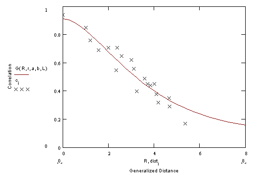
Fig. 1. Fitting of the correlation function to sample data.
The equation for the z-t residuals is formulated by conventional optimal interpolation for the point i, as:
![]() (4)
(4)
with weights, W, given by
![]() (5)
(5)
with
 (6)
(6)
in which cij is the modeled correlation between points i and j, and e is the assumed ratio of observation error variance to 6-hour forecast error variance. (Note that I is the vector of increments and not the identity matrix.) The data used in the solution are the closest 9, as defined by (2), to the observation point (i.e. n = 9).
b. Decision Making Algorithm
Decisions on data quality are made by the Decision Making Algorithm which makes specific use of the assumptions regarding the various data types as enumerated above.
All winds with speed less than 1 ms-1 are marked as bad.
The determination of influence of bird migration on the VAD winds follows the methodology used for the profiler winds. No bird migration is assumed to occur except between 15 February and 15 June for the spring migration, and between 15 August and 15 November for the fall migration. Within the migration dates, a wind is considered to be likely influenced by bird migration if the forecast temperature is above –3 C, and the v-component of the wind increment is above 8 ms-1 in magnitude, from the south in the spring and from the north in the fall. All such winds are marked as bad.
Fig. 2. Shows all wind increments between 899 and 850 hPa for 06 UTC 1 March 2000. Most of the wind v-component increments exceed 8 ms-1 in the southeast U.S. and into the upper mid-west. These very likely reflect the nighttime maximum in bird migration. Many of these winds were marked so that they would not be used.
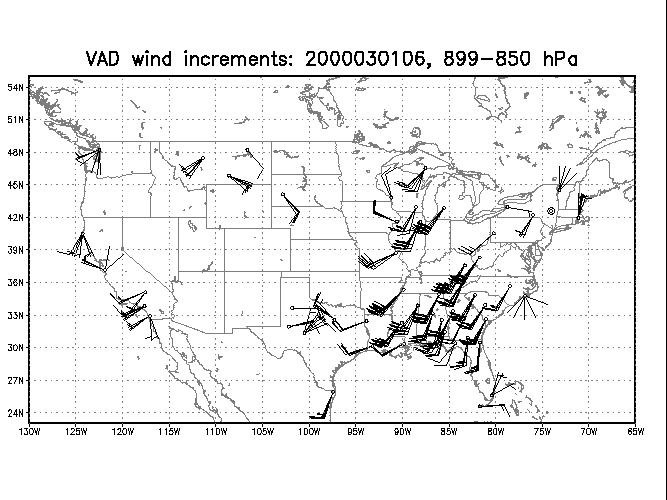
Fig. 2. Sample VAD wind increments.
The rough errors are assumed to be of nearly any magnitude and superimposed on small random errors with zero mean. By specifying the expected proportion of data to contain rough errors, and the range that they may have, it is possible to formulate the expected ‘weight’ that these observations would have in a variational analysis. Fig. 3 shows a sample weight function.
The weight is calculated separately for the speed increment and z-t speed residual for data at a specific height, and the height immediately below. The magnitude of the sum of the weights for the speed increment and z-t speed residual for the specific height, w0, and the sum of the weights for the level below, w1, are used to determine the likelihood of rough errors. If w0 is less than 0.3, then the wind is marked as bad (both u and v), and if w0 and wl are both less than 0.55, the winds at both levels are marked as bad. These specific limits are chosen by experiment, but the weight function has a rather sharp cutoff, so that the exact values of these constants is not critical. It is important, however, that the sum of the increment and z-t residual weights be used in these tests as this guarantees that the individual weights both be small for a rough wind to be diagnosed. This helps to keep large increments, by themselves, from causing winds to be marked as bad, but as a safety measure, all winds with a wind component increment greater than 12 ms-1 are marked as bad.
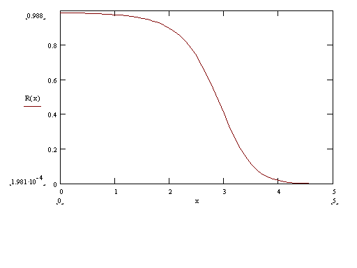
Fig. 3. Weight function for VAD rough errors, where x is the residual, normalized by subtracting the mean and dividing by the standard deviation, and R is the weight. It was assumed that 7% of the data contain rough errors.
5. Performance of the quality control algorithm
The number of errors found in any 6-hour time period can vary significantly. Fig. 4. shows the count of errors for the first eight days of March, 2000, divided into 6-hour time periods, centered about the main observation times of 00, 06, 12 and 18 UTC and Fig. 5 shows the errors as a percentage of all winds received.
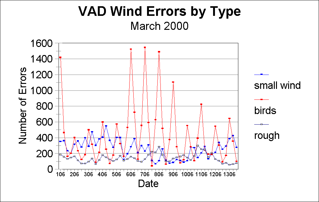
Fig. 4. Count of VAD wind errors by error type, for 6-hour time periods centered on the main observation times of 00, 06, 12 and 18 UTC, for first 13 days of March, 2000.
In the figures, the wind errors are broken into: winds of small magnitude, winds likely influenced by bird migration, and winds containing rough errors. This latter category contains three sub-types that have been lumped together.
Clearly, the greatest variability in diagnosed errors is in those influenced by bird migration, with counts as low as about 100 and as high as 1500. The maximum is always for the time period centered on 06 UTC, and its value has large changes, possibly due to sampling variations. Check against weather maps did not show any obvious relationship between the periods of fewer ‘bird’ winds and unfavorable winds.
Next in importance for quality control are the winds of small magnitude, comprising about 100-550 or 2-15% of the total for any 6-hour period. One possible explanation might be that these winds are contaminated by ground return, but that seems unlikely since they are present for winds at all heights. The few good winds of small magnitude are lost to our use since they also are marked as bad.
The rough errors occur least frequently, comprising about 150 or 3-4% for each six hours. The source of these errors is not known, but would include any failure of the Doppler wind algorithms to deal with range and velocity ambiguities, and any large wind errors due to model guess or nonrepresentativeness. If they are possible, any communication errors would also be included.
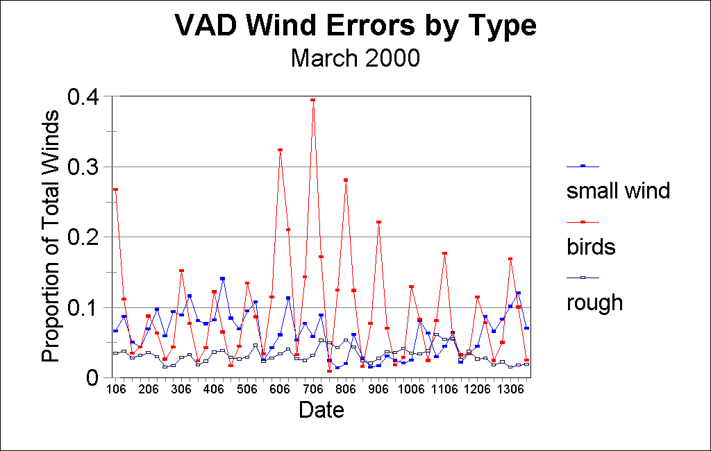
Fig. 5. VAD wind errors by error type, as a percentage of the total winds received for 6-hour time periods centered on the main observation times of 00, 06, 12 and 18 UTC, for the first 13 days of March, 2000.
6. Acknowledgments
This work was done with the strong support of EMC, and particularly Geoffrey DiMego. The data was made available in a format for easy quality control by Dennis Keyser. Discussion with Dave Parrish, who has used the radar winds in 3-dimensional variational analysis as radial winds, was very valuable.
References
Browning, K.A. and R. Wexler, 1968, The determination of kinematic properties of a wind field using Doppler radar, Journal of Applied Met., 7, 105-113.
Collins, WG, 1993: Complex quality control of Doppler wind profilers at the National Meteorological Center, 13th Conference on Weather Analysis and Forecasting, Aug. 2-6, 1993, Vienna, VA.
__________, 1994: Complex quality control of wind profiler data at the National Meteorological Center, Tenth Conference on Numerical Weather Prediction, July 18-22, 1994, Portland, OR.
Lhermitte, R.M. and D. Atlas, 1961: Precipitation motion by pulse Doppler, Proc. 9th Weather Radar Conference, Kansas City, AMS, 218-223.