The Identification of Observation Errors in Radiosonde Mass Data at the National Centers for Environmental Prediction
William G. Collins
NCEP/Environmental Modeling Center
Washington, DC
The complex quality control for radiosonde heights and temperatures is made by the prepbufr_cqcbufr program at the National Centers for Environmental Prediction (NCEP). The program diagnoses many errors, and some it can correct. The errors that it deals with are called ‘rough’ errors since their statistical distribution contains a component that is reasonably uniform, and definitely not normally distributed as would be expected for instrument errors or errors of non-representativeness. These rough errors are classified as communication errors, computation errors, and observation errors. A new algorithm for the diagnosis of these observations errors is the subject of this paper. Most of cqcbufr is concerned with the diagnosis and possible correction of communication and computation errors. These errors are generally detectable by a complex of hydrostatic inconsistencies between observation levels. The observation errors—the subject of this note—never lead to hydrostatic inconsistencies. The use of the term ‘observation error’ needs some explanation. It is used strictly to mean those errors that cannot be detected by hydrostatic inconsistencies, but have sufficient magnitude to require identification for non-use in the assimilation of data. As such, these errors are not the same as instrument error, but include instrument error as a component. They include errors from any cause that precedes the computation of heights from the temperatures and moisture.
Within the framework of numerical analysis, Lorenc and Hammon (1988) study the quality control process in terms of Bayesian probability theory, in which "the error in each datum is either a normal observation error, from a known Gaussian distribution, or a gross error, in which case the datum gives no information". In the present note, what was defined above as "observation error" will be considered to contain the two parts considered by Lorenc and Hammon: 1) instrument and other errors with Gaussian distribution, and 2) rough observation errors with (assumed) uniform distribution. The method of performing the quality control of these data by cqcbufr closely follows the development of Schyberg and Breivik (1997), who made the same assumptions.
2. General description of cqcbufr
The cqcbufr is documented in Collins (1998, 2000?) . Here only a broad outline will be given, especially as it is relevant to the quality control of observation errors (as defined in Section 1). The data are read in for a first time and all residuals are calculated. The residuals are: 1) increments (difference between the observed value and the 6-hour forecast value), 2) vertical residuals (difference between the increment and vertically interpolated increment, using statistical interpolation), 3) horizontal residuals (difference between the increment and horizontally interpolated increment, using statistical interpolation), 4) hydrostatic residuals (difference between a layer thickness, computed by heights and by temperatures and moisture), 5) baseline residual (a form of hydrostatic residual), and 6) lapse rate residuals.
For use by the observation error detection algorithm, the residuals are converted to normal standard deviates:
![]() , (1)
, (1)
where ![]() is the normalized residual for type t (1-3 above),
is the normalized residual for type t (1-3 above), ![]() is the residual value,
is the residual value, ![]() is its mean, and
is its mean, and ![]() is its standard deviation. The mean and standard deviation are determined from all the data for the present data time in which a crude attempt is made to eliminate from the computation, data that very likely have a large rough error. In other words, the mean and standard deviation used in the normalization are supposed to represent values appropriate to the part of the error distribution that has a Gaussian distribution.
is its standard deviation. The mean and standard deviation are determined from all the data for the present data time in which a crude attempt is made to eliminate from the computation, data that very likely have a large rough error. In other words, the mean and standard deviation used in the normalization are supposed to represent values appropriate to the part of the error distribution that has a Gaussian distribution.
The data are then read in a second time, one report at a time. The full power of the Decision Making Algorithm (DMA) is used to examine a complete profile of data for communication and computation errors. Only when the complete profile has been examined, and any possible corrections are made, will the DMA examine the data for observation errors. The remainder of this note will discuss that examination, under the assumption that the observation errors are composed of the two parts as discussed above—a part with Gaussian distribution (with parameters now known) and a part with (assumed) uniform distribution.
As the data are read in, statistics are collected on the three residuals: increment, vertical residual and horizontal residual. In this collection, large values are eliminated, so that the mean and standard deviation values obtained may be reasonably assigned to the Gaussian part of the error distribution. Values of mean and standard deviation are obtained for the radiosonde heights, temperatures, and dew-point temperatures at each mandatory level.
The second part of the observation error distribution consists of the rough errors. The number of these errors may be estimated from an earlier version of the cqcbufr and then modified as required. All that is needed is an estimate of the proportion of the data containing such errors, and a range over which such errors are likely. The probability distribution for observation errors may thus be given by
![]() , (2)
, (2)
where ![]() is the probability that a value does not contain a rough error,
is the probability that a value does not contain a rough error, ![]() is the probability that a value does contain a rough error,
is the probability that a value does contain a rough error, ![]() is the Gaussian distribution for the normalized residual
is the Gaussian distribution for the normalized residual ![]() , and C is given by
, and C is given by
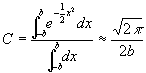 , (3)
, (3)
in which rough errors are assumed to be contained within ![]() 2b standard deviations of the mean.
2b standard deviations of the mean.
The lower curve in Fig. 1 shows the combined error distribution, assuming that 5% of the data contain rough errors and that they extend over 5 standard deviations with regard to the Gaussian part of the distribution.
A datum may contain an observation error of sufficient magnitude that it should be marked as bad either because it is part of the Gaussian distribution, out on its tail, or that it is a rough error of large size. The formulation of Schyberg and Breivik gives a weight that a datum should have for an analysis, in the presence of the assumed error distribution. The upper curve in Fig. 1. shows this weight with the assumed parameter values. Note that it remains near a value of 1. out to 2 standard deviations, but falls rapidly toward 0. between 2.5 and 3.5 standard deviations. The weight, ![]() , is given by
, is given by
![]() . (4)
. (4)
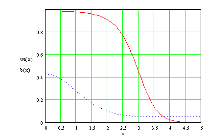
Fig. 1. "Analysis weight" (upper curve) and error distribution (lower curve) under the assumption that the rough errors comprise 5% of the data, and are distributed over 5 standard deviations with regard to the Gaussian part of the error distribution.
The cqcbufr computes a weight individually for the increment, vertical residual and horizontal residual for each datum. The next section will discuss the specifics of use of these weights in specifying data with observation errors.
Each of the analysis weights for a particular datum gives an estimate of the value of the data for assimilation. Recognizing that there may be an inconsistency between the (at most) three weights, the cqcbufr uses an average of the weights in its determination. This average can only be small if all weights agree that the datum is bad.
First, there is examination to see if a datum is given a "keep" flag by manual intervention. If so, the datum is not considered eligible for an observation error, rather deferring to human judgment. Then the weight average is used to determine the observation class:
|
|
datum has no observation error |
|
|
datum is questionable (given quality flag 3.) |
|
|
datum is bad (given quality flag 13.) |
Whenever a datum is found to be questionable or bad a quality mark is written to the prepbufr file to identify this fact. This observation error determination is made for radiosonde heights, temperatures and dew-point temperature.
Observation errors are quite common, but only a few examples will be given. In the first example, the temperatures at three levels
were marked as bad because of observation errors. In the tables below, the shorthand shown below will be used.
In the second example, the height at a single level is flagged since the residuals are excessive in size. And in the last example, the top level height is flagged as bad. All three of these examples are typical.
|
****FOR TEMPERATURE*** |
***FOR HEIGHT*** |
|||||
|
P |
pressure |
P |
Pressure |
|||
|
TOB |
observed temperature |
ZOB |
observed height |
|||
|
TI |
temperature increment |
ZI |
height increment |
|||
|
TV |
T vertical residual |
ZV |
height vertical residual |
|||
|
ZH |
height horizontal residual |
|
|
|||
|
XTI |
normalized TI |
XZI |
normalized ZI |
|||
|
XTV |
normalized TV |
XZV |
normalized ZV |
|||
|
XZH |
normalized ZH |
|
|
|||
|
ACP |
analysis weight |
ACP |
analysis weight |
|||
|
QM |
quality mark |
QM |
quality mark |
|||
Table 1. Temperature observation errors for 35700 at 00 UTC 21 March, 2000.
|
P |
TOB |
TI |
TV |
XTI |
XTV |
ACP |
QM |
|
637 |
-.7 |
11.3 |
6.3 |
7.2 |
8.0 |
.000 |
13 |
|
621 |
.2 |
13.6 |
9.8 |
8.6 |
12.3 |
.000 |
13 |
|
543 |
-31.7 |
-10.8 |
-8.0 |
-6.8 |
-10.0 |
.000 |
13 |
Table 2. Height observation error for 56096 at 00 UTC 21 March, 2000.
|
P |
ZOB |
ZI |
ZV |
ZH |
XZI |
XZI |
XZH |
ACP |
QM |
|
500 |
5570 |
-103 |
-76 |
-112 |
-6.6 |
-10.5 |
-7.6 |
.000 |
13 |
Table 3. Height observation error for 48455 at 00 UTC 21 March, 2000.
|
P |
ZOB |
ZI |
ZV |
ZH |
XZI |
XZI |
XZH |
ACP |
QM |
|
70 |
18310 |
-277 |
-255 |
-243 |
-5.6 |
-12.2 |
-6.5 |
.000 |
13 |
|
|
|
|
|
|
|
|
|
|
|
Statistics are collected from the routine running of cqcbufr to summarize them on a monthly basis. Some information has been extracted on the observation errors detected during February, 2000, in which there were 31760 radiosonde reports collected at NCEP. There were 1773 observation errors detected, of which 217 received quality mark 3 (questionable) and 1556 received quality mark 13 (bad). By contrast, the presently operational code diagnosed 11,463 data with observation errors, with 9480 given quality mark 3 and 1983 give quality mark 13. The new observation error quality control makes more definitive decisions and slightly reduces the number of "bad" quality marks. In pressure, the largest number were at
1000 hPa, with counts trailing off in height. (A minimum value at 925 hPa is likely caused by fewer observations reporting this level.)
The geographic distribution is far from uniform, and is given in Table 4. for the major regions of the globe.
Table 4. Distribution of observation errors by large region for February 2000
|
Western Europe |
45 |
|
Eastern Europe |
42 |
|
Former USSR |
83 |
|
Western Asia |
27 |
|
India, Ceylon |
435 |
|
Mongolia |
6 |
|
Taiwan, Korea, Japan |
18 |
|
Indochina, Malaysia |
27 |
|
China |
401 |
|
N. and Central Africa |
139 |
|
South Africa |
7 |
|
United States |
33 |
|
Canada |
27 |
|
Central America |
49 |
|
South America |
113 |
|
Antarctica |
63 |
|
Pacific |
172 |
|
Australia, New Zealand |
7 |
The absolute numbers of errors detected is not of primary importance since this can be tuned to some extent by the choice of various parameters. It was the objective to let the data itself determine them as much as possible, and manual examination of the results looks reasonable. In many respects, the result is statistical and one should not expect 100% accuracy. There are bound to be many cases in which bad data are not flagged and many other cases in which good data are flagged. The great majority of the decisions, however, appear to be correct. Using very small values of the mean analysis weight for flagging data as bad is conservative; there are probably more bad data accepted than good data rejected.
References
Collins, W.G., 1998: The use of complex quality control for the detection and correction of rough errors in rawinsonde heights and temperatures: a new algorithm at NCEP/EMC. NCEP Office Note 419. [Available from NCEP, 5200 Auth Road, Washington, D.C. 20233.]
___________, 2000?: The operational complex quality control of radiosonde heights and temperatures at the National Centers for Environmental Prediction: Part I. Description of the method. Submitted to Journal of Applied Meteorology.
___________, 2000?: The operational complex quality control of radiosonde heights and temperatures at the National Centers for Environmental Prediction: Part II. Examples of error diagnosis and correction and statistics of error determination for a year in operational use. Submitted to Journal of Applied Meteorology.
Lorenc, A.C. and O. Hammon, 1988: Objective quality control of observations using Bayesian methods. Theory, and a practical implementation. Q.J.R. Meteorol. Soc., 114, pp. 515-543.
Schyberg, Harald and Lars-Anders Breivik, 1997: Objective analysis combining observation errors in physical space and observation space. Research Report No. 46, Norwegian Meteorological Institute, 35 pp.