The present NCEP Regional assimilation system uses elements of quality control (qc) that are specific to particular data types. It uses individual qc codes for radiosonde temperatures and heights, aircraft observations, profiler winds, and VAD winds. The Regional system does not use a general optimal interpolation qc (oiqc) as does NCEP's Global assimilation system, but rather presently only has a check on gross data errors.

Variational analysis operates by searching for a minimum to an objective function which measures the square difference of the analysis from all observations and the background (6-hour forecast) state, where the fit is weighted according to the observation and background error statistics. All data mutually influence each other in both the analysis and qc through the observation and background objective functions. The solution for the objective function is iterative, allowing the possibility for qc of the data which adapts to the estimate of the analysis at each iterative step (Ingleby and Lorenc, 1993).

The qc is based upon Bayesian probability theory (Lorenc and Hammon, 1988). The data is assumed to contain a non-Gaussian (gross) component in addition to the usual Gaussian error distribution. In this formulation the observation errors are assumed to be uncorrelated, an assumption which is not strictly correct for all data types, e.g. radiosonde heights and satellite radiances. The gross error component is assumed to have a flat distribution within some number of standard deviations from the mean. This leads to a modification to the observation part of the objective function which effectively gives data which are far from the analysis a reduced weight.

This paper gives the analysis equations, highlighting how they differ because of the inclusion of the gross error component and its quality control. The formulation follows closely that suggested by Schyber and Breivik (1997) and Andersson and Järvinen, 1998. Distributions of analysis increment for each variable type are discussed and the impact of the quality control is illustrated for a single case. This quality control is scheduled for operational implementation at NCEP in late September, 2000.

The 3dvar minimizes the difference between the analysis and its fit to the observations, background (6-hour forecast), and physical constraints. This is expressed by minimization of the objective function

where the background part of the objective function is given by

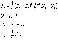
In this notation, variables with a tilde refer to the original unscaled, dimensional variables. The subscript a refers to analysis variables and the subscript b refers to the background. is the background error correlation matrix. The observation part of the objective function is given by

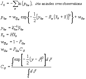
where is the observation, variables with an overbar are at the observation location, R is a normalized non-linear operator needed for some observation types, e.g. wind speed, is the observation error, and H is the combined interpolation operator and linear part of the forward model.

The weight is the probability that a datum does not have a gross error. When i.e. no gross error, then the observation contribution to the objective function has its usual form

The solution for the minimum of J is performed by a descent algorithm in which the effective weight given to a datum depends upon its fit at the present stage in the descent solution and by the assumed probability of gross error. In this way, the quality control is said to be non-linear. The effective analysis weight given to a datum is

Again, with the assumption of no gross error, the effective analysis weight is 1. With a more usual assumption of gross error in 5% of the data, the weight as a function of (called simply x in the figure) is shown in Fig. 1. Also shown in the figure is the assumed error probability distribution. It is the normal distribution with .05 added over the range of . The assumption is that the gross errors, while they may be large, are nevertheless limited (to 5 times the standard deviation of normally distributed observation errors).

The cutoff in the effective analysis weight is seen to be rather sharp, so that data within 1.5 standard deviations get a weight near 1., while data farther from the mean than 4.0 standard deviations get very small weight.

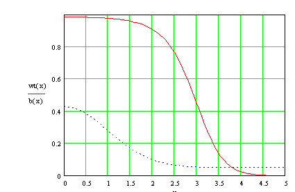
Fig. 1. Effective analysis weight (solid curve) and probability distribution (dotted curve) as a function of the difference of the observation from the 3dvar solution.

The weight given in the 3dvar analysis to a datum is determined to some degree by the values chosen for the probability of gross error and the range over which gross errors are assumed to occur. However, the analysis weight is much more strongly determined by the values of observation error used, determining the normalization of . One would suspect that the standard deviation of this quantity would be 1.0, since this is a normalized quantity, but the standard deviation varies for each data type. For moisture (q), it is about 0.25, for temperature 0.58, for height 0.47, for precipitable water 0.05, and for winds 0.45. Since these are all less than 1.0, the analysis weights are increased from what they would otherwise be. This also lessens the number of data that are flagged as bad for a particular weight limit. Figs. 2-6 show the distribution of for the various variables.

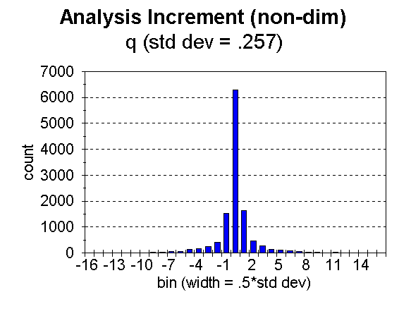
Fig. 2. Distribution of analysis increment, , for bins of width = 0.5 times the standard deviation, for specific humidity.

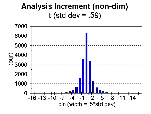
Fig. 3. Distribution of analysis increment, , for bins of width = 0.5 times the standard deviation, for temperature.

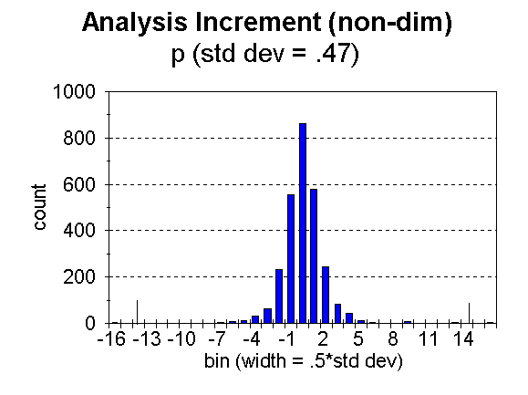
Fig. 4. Distribution of analysis increment, , for bins of width = 0.5 times the standard deviation, for height.

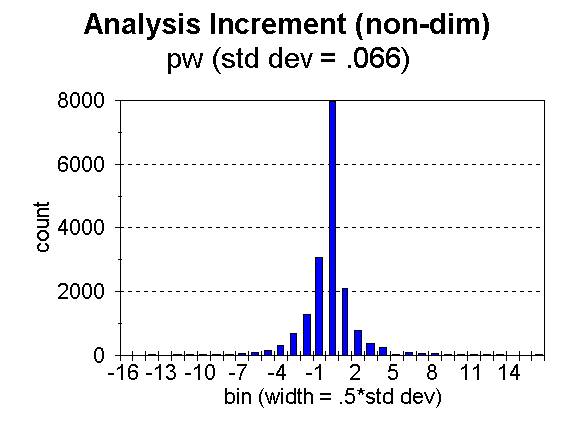
Fig. 5. Distribution of analysis increment, , for bins of width = 0.5 times the standard deviation, for precipitable water.

Fig. 6. Distribution of analysis increment, , for bins of width = 0.5 times the standard deviation, for wind components.

The number of moisture data flagged (i.e. noted as likely bad) in this case was 1 out of 11,701. A total of 38 temperatures, out of 18,874 were flagged, 11 out of 2,755 heights, and 57 out of 64,962 winds. The limiting analysis weight for noting a datum to be likely bad was 0.5. In the figures, the approximate limits are noted (for t, p, and w) by tick marks along the abscissa. This number of bad data seems unusually small, but as stated, the number is strongly influenced by the values of observation error used. It must also be remembered that NCEP’s Regional 3dvar is used over the United States and surroundings, a region of good data quality.

The impact of the quality control may also be determined from examination of the difference between analyzed 3dvar analysis fields from runs with and without the non-linear quality control. Such a comparison is shown in Figs. 7 and 8 for the important snow case following 12 UTC 24 January 2000. Fig. 7 shows the pressure difference at sea level, and Fig. 8 shows the height difference at 500 hPa. It is seen that the differences over western Minnesotta and Quebec are barotropic in the vertical. Observations (not shown) support the analysis with the non-linear quality control. In this particular case, these differences do no appear to be reflected in forecast improvement; in fact, there is little difference downstream from these regions, even at 12 hours.

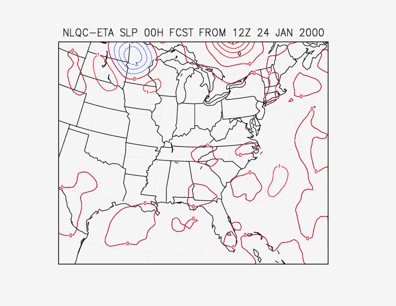
Fig. 7. Sea level pressure difference between analyses with and without non-linear quality control, for 12 UTC 24 January, 2000.

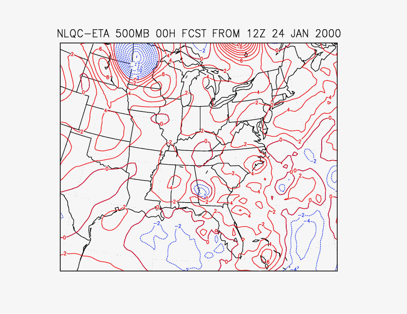
Fig. 8. 500 hPa height difference between analyses with and without non-linear quality control, for 12 UTC 24 January, 2000.

References

Schyberg, Harald and Lars-Anders Breivik, 1997: Objective analysis combining observation errors in physical space and observation space, Research Report No. 46, Det Norske Meterologiske Institutt, Oslo, August 20, 1997, 35pp.
Ingleby, N.B. and Lorenc, A.C., 1993: Bayesian quality control using multivariate normal distributions. Q.J.R. Meteorol. Soc., 119, 1195-1225.
Lorenc, A.C. and Hammon, P., 1988: Objective quality control of observations using Bayesian methods. Theory, and a practical implementation. Q.J.R. Meteorol. Soc., 114, 515-543.
Schyberg, H. and Breivik, L., 1997: Objective analysis combining observation errors in physical space and observation space, Norwegian Meteorological Institute, Research Report No. 46, 35 pp