ON THE ABILITY OF ENSEMBLES TO DISTINGUISH BETWEEN FORECASTS WITH

SMALL AND LARGE UNCERTAINTY

Zoltan Toth¹, Yuejian Zhu¹, and Timothy Marchok¹
National Centers for Environmental Prediction

Submitted to
Weather and Forecasting

Revised
February 22, 2000

¹General Sciences Corporation (Beltsville, MD) at NCEP

^{Corresponding author's address: Zoltan Toth, NCEP, Environmental Modeling Center, 5200 Auth Rd., Room 207, Camp Springs, MD 20746
e-mail: Zoltan.Toth@noaa.gov}

ABSTRACT

In the past decade ensemble forecasting has developed into an integral part of numerical weather prediction. Flow dependent forecast probability distributions can be readily generated from an ensemble, allowing for the identification of forecast cases with high and low uncertainty. The ability of the NCEP ensemble to distinguish between high and low uncertainty forecast cases is studied here quantitatively. Ensemble mode forecasts, along with traditional higher resolution control forecasts, are verified in terms of predicting the probability of the true state being in one of 10 climatologically equally likely 500 hPa height intervals. A stratification of the forecast cases by the degree of overall agreement among the ensemble members reveals great differences in forecast performance between the cases identified by the ensemble as the least and most uncertain. A new ensemble based forecast product, the "relative measure of predictability", is introduced to identify forecasts with below and above average uncertainty. This measure is standardized according to geographical location, the phase of the annual cycle, lead time, and also the position of the forecast value in terms of the climatological frequency distribution. The potential benefits of using this and other ensemble based measures of predictability is demonstrated through synoptic examples.

1. Introduction

During the past decade, ensemble forecasting has become an integral part of numerical weather prediction (NWP). Major meteorological centers now regularly produce and use ensemble forecasts (Molteni et al. 1996; Toth and Kalnay 1993; Rennick 1995; Houtekamer et al. 1996; Kobayashi et al. 1996). The role of ensemble forecasting will likely expand in the coming years within the National Weather Service where the use of probabilistic weather, water and climate forecasts has been adopted as one of the strategic goals to be achieved by 2005 (NWS 1999). One of the main advantages of ensemble forecasting is that it can potentially provide case dependent estimates of forecast uncertainty (Ehrendorfer 1997). To what extent this promise is fulfilled by the current NCEP global ensemble forecast system (Toth and Kalnay 1997) is the main topic of the present study.

The generation and verification of probabilistic forecasts based on ensembles was the subject of a number of recent studies (e. g., Anderson 1996; Hamill and Colucci 1997; Talagrand et al. 1997; Eckel and Walters 1998; Atger 1999; Richardson 2000). General statistics for the performance of the NCEP ensemble forecasting system were provided by Zhu et al. (1996, with a comparison to that of the ECMWF Ensemble Prediction System), and Toth et al. (1998, with a comparison to that of a single higher resolution control forecast). These earlier studies demonstrated that the ensemble forecasts can be used to generate skillful probabilistic forecasts, which, after a simple statistical postprocessing based on verification statistics from the recent past, become very reliable.

In recent studies (Mylne 1999; Richardson 2000; and Zhu et al. 2001) it was also demonstrated that the potential economic value associated with the use of an ensemble forecasting system may be considerably greater than that attainable by using a single, even higher resolution control forecast, given substantial uncertainty in the forecasts (i. e., 500 hPa height forecasts at and beyond 3 days). Note that in the above comparisons neither the ensemble nor the control forecasts were statistically corrected or postprocessed. It was also shown (Toth et al. 1998) that the extra value associated with an ensemble of forecasts as compared to a single control forecast is due to two main factors: (1) the ensemble can characterize foreseeable, flow dependent variations in the uncertainty of the forecasts; and (2) the ensemble can provide a probability distribution that is more complete than a dichotomous probability description given by a single forecast.

With appropriate postprocessing using past verification statistics, a full probability distribution can be generated from a single control forecast (see, e. g., Talagrand et al. 1997; Talagrand 1999, personal communication). Talagrand's results indicated, however, that postprocessed full probabilistic forecast distributions based on a single control forecast still did not reach the resolution skill level of that provided by a statistically uncorrected ensemble of forecasts, attesting to the value of case dependent uncertainty information provided by the ensemble. In a recent study, Atger (2001) attempts to render case dependent variations in forecast uncertainty to a single forecast, depending on its spatial and temporal structure. If and to what degree such a statistical approach can compete with an ensemble of forecasts based on the estimated initial value uncertainty and its dynamical evolution (Ehrendorfer 1997) is to be evaluated.

In this paper we investigate the extent to which an ensemble of forecasts can distinguish between forecast situations with lower or higher than average expected uncertainty, based on their flow dependent level of similarity or dissimilarity. Ensemble forecasts over a period of a season (section 2) will be stratified according to the degree of ensemble forecast similarity (section 3). The main results of this study will be presented in section 4. Based on these results, section 5 introduces a new forecast product, the "relative measure of predictability". In section 6, the use of different measures of predictability is demonstrated through synoptic examples, while the conclusion and discussion are given in section 7.

2. Ensemble forecast data

In the present study, the NCEP operational global ensemble forecasts (Toth and Kalnay 1997) will be evaluated over the period March - May 1997. The aim here is to assess the extent to which ensemble forecasts can distinguish between cases of higher or lower than average uncertainty. The studied period is from a transition season that coincides with that of Toth et al. (1998). Note that predictability in a transition season is typically lower than in winter but higher than in summer.

The NCEP global ensemble forecasts in 1997 consisted each day of 17 individual forecasts run out to 16 days lead time, of which 3 were control forecasts started from unperturbed analyses, and 14 were perturbed forecasts started from initial conditions where bred perturbations of the size of estimated analysis uncertainty were both added to, and subtracted from the control analyses at 0000 and 1200 UTC (Toth and Kalnay 1997). In section 4, the 14 T62 resolution perturbed forecasts (10 from 0000 UTC, and 4 from 1200 UTC) are evaluated, along with the 0000 UTC MRF T126 high resolution control forecast that provides a reference level of skill.

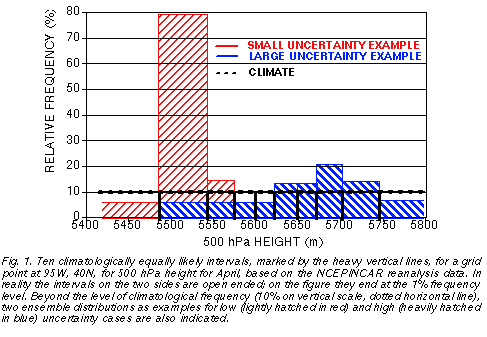
500 hPa height forecast and analysis data will be used over the Northern Hemisphere (NH) extratropics (20N - 77.5N), on a 2.5 by 2.5 latitude-longitude grid. As in Zhu et al. (1996), and Toth et al. (1998), the forecast and verifying analysis data will be binned at each grid point into 10 climatologically equally probable intervals (Fig. 1). These intervals were defined uniquely for each grid point and each month of the year using the NCEP reanalysis data (Kalnay et al. 1996). They were then linearly interpolated in time to each date within the study period.

3. Methodology

a. Stratification by expected uncertainty

On each day and at each grid point in the period and region studied, the distribution of the 14 ensemble forecasts at each lead time is evaluated in terms of the 10 climatologically equally likely bins. In particular, the number of ensemble forecast members associated with the most highly populated climate bin is noted. The population in this bin is the mode (m) of the ensemble distribution, and its value for a 14-member ensemble given in 10 climatologically equally likely bins varies between 2 and 14. The frequency distribution of the mode values over all grid points and all case days is denoted by f(m). High ensemble mode values (14, or close to 14) correspond to a compact ensemble, where most members indicate very similar height values, whereas low ensemble mode values (2, or close to 2) indicate a diverse ensemble with little agreement among the members. The former cases generally represent forecast situations with a small ensemble spread, with presumably small forecast uncertainty, while the latter cases are characterized by large ensemble spread, presumably indicating high forecast uncertainty (see two forecast distribution examples in Fig. 1).

To evaluate the ability of the ensemble to distinguish between forecast cases with low and high uncertainty, 10-15% (P=0.1-0.15) of the total number of cases (over all grid points and days) associated with the highest and lowest ensemble mode values are identified for all lead times. This is achieved by selecting all grid points separately for which m<M_l (presumed low predictability) and: and for which m>M_h (presumed high predictability) and:At short lead times the ensemble spread is generally small, and thus M_h is typically large (close or equal to 14). As the lead time increases, the ensemble spread also increases and consequently M_h decreases. For the subset of cases with the lowest ensemble mode, at long lead time, M_l=2 or only slightly higher. At shorter lead times with concomitantly smaller ensemble spread, M_l must be larger to account for approximately the same fraction (10-15%) of all cases.

b. Measure of performance

The 10-15% of cases with the highest and lowest ensemble mode values will be referred to as the "low uncertainty" (or high predictability), and "high uncertainty" (or low predictability) cases respectively. Charts outlining the geographical areas associated with these cases can be made available in real time to the forecasters (see section 5). The main results of this study shown in the next section pertain to the performance of categorical ensemble mode forecasts, evaluated separately for the high and the low predictability cases as defined above. In addition, the average performance of the control MRF forecasts, which without statistical postprocessing cannot be objectively classified into high or low predictability cases, will also be evaluated. The performance measure used for evaluating both the ensemble mode and MRF control forecasts is the average success rate of the particular categorical forecast system:

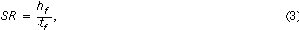
where h_f is the number of cases (hits) when a forecast system, calling for the occurrence of a particular climate bin, correctly verified, and t_f is the total number of all such forecasts, accumulated over all climate bins. In section 4 success rate results for the MRF control forecast (averaged over all cases), and for ensemble mode forecasts evaluated separately over the high and low predictability cases, will be shown. Note that when there are more than one climate bins associated with the value of the ensemble mode, the verification result for one such bin, selected arbitrarily among them, will be included in the statistics.

The success rate as defined above is the complement of the false alarm rate (SR=1-FAR) and is called postagreement in the older literature (see Wilks 1995). In general the performance of a system forecasting a particular event (any one particular bin out of 10 climate bins) can be described by a 2x2 contingency table (defined by yes/no alternatives for both forecast and observed events), or alternatively, three independent measures based on such a table. Since the event to be predicted in our case has a climatological frequency of 0.1, and the overall forecast frequency of any particular bin (barring any significant model bias) is also 0.1, the success rate (Eq. 1) uniquely describes the performance of the forecast systems when integrated over all 10 climate bins. If the ensemble mode forecasts exhibit resolution, case dependent probabilistic categorical forecasts can be issued (section 5).

c. Attributes of probabilistic forecasts

The two main attributes of probabilistic forecasts are their reliability and resolution (see, e. g., Stanski et al. 1989). Reliability implies that forecast probability values match the conditional observed frequencies of the same events over the long run, e. g., forecasts issued with a 40% probability verify 40% of the time. Reliability, however, does not necessarily imply value. For example, if the climate probability of the predicted event is also 40%, the forecast would not have value with respect to using climatological information only. Assuming perfect reliability, resolution is a measure of how "sharp" the probabilistic forecasts are, i. e., how close the forecast probability values are to the ideal 0 and 1 values. Perfect resolution (i. e., the exclusive use of 0 and 1 probability values, as with the use of a single control forecast), however, does not guarantee optimal forecasts either, unless accompanied by perfect reliability. An ideal probabilistic forecast system in fact has as much resolution as possible, while exhibiting perfect reliability at the same time.

We know from earlier verification studies (e. g., Zhu et al. 1996; Toth et al. 1998) that probabilistic forecasts based on an ensemble (or a control) forecast can be easily calibrated to make them very reliable. Probability values based on the relative frequency of ensemble members indicating a particular weather event (say, 6 out of 10 members forecasting one of the 10 climatologically equally likely bins) may be adjusted to match the past observed frequency of that event, given the same (in this example, 6) ensemble forecast frequency of the weather event. Calibration amounts to a bias removal in the probability space and can be used to reduce the effect of model bias and insufficient ensemble spread as long as the system behaves consistently in time.

While ensemble-based probabilistic forecasts can be made almost perfectly reliable through calibration, resolution cannot be improved in such a trivial manner. In this study we evaluate how much resolution ensemble mode forecasts have in terms of their ability to distinguish between forecast cases with low and high uncertainty, based on extremely low and high mode values. Since postagreement (success rate) is used in the next section to evaluate the ensemble's ability to distinguish between low and high uncertainty categorical forecasts, the reliability of probabilistic forecasts is not considered in the analysis presented in the next section. Reliability and calibration will, however, be discussed in sections 5 and 6 where probabilistic (instead of categorical) forecasts will also be considered.

Let us assume that every time the same set of probability values are used for predicting the 10 climate categories used in this study, except arranged in different ways over the 10 categories. Standard measures of resolution (e. g., the resolution part of the ranked probability skill score, RPSS, see, e. g., Wilks 1995) would indicate a certain amount of resolution , depending on how different the 10 probability values are from the climatological probability value (10%). Such a forecast system would not be able to distinguish between forecast cases with different degrees of predictability. The resolution in such a system can be termed internal to the probability distribution used. The issue of case (as opposed to the more trivial distribution) dependent resolution can only be addressed with an experimental setup similar to that used in this study, where the uncertainty associated with a forecast for a single category or event is analyzed. If case dependent resolution is found, the difference in success rates for the low and high uncertainty cases also provides an easily comprehensible measure of this characteristics of the ensemble. In contrast, values of RPSS scores and other alternative measures are not as straightforward to interpret.

4. Results

As a function of lead time, Fig. 2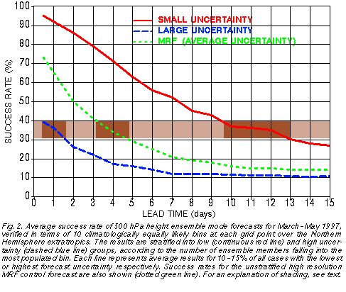 evaluates how different the success rates of the forecasts are for the 10-15% of all cases with the lowest and the highest predictability, as identified in real time by the ensemble. The average success rate for all cases, using the MRF control forecast, is also shown. Note that the ensemble mode forecasts evaluated for all cases without stratification (not shown) exhibit success rates similar to that of the high resolution control, except with somewhat lower values before, and somewhat higher values after day 6 lead time (see Fig. 3 of Toth et al. 1998).

The results indicate that the ensemble forecasting system that was operational in the spring of 1997 had a substantial case dependent resolution. For example, at 1 day lead time the 10-15% of most predictable forecasts verified with a success rate of 92%, while the least predictable 10-15% verified with a success rate of only 36%. The average success rate for the unstratified MRF forecasts was 65%. The verification statistics at later lead times reveal a somewhat reduced, but still wide range of success rates. While the overall MRF success rates at 4 (12) day lead time are 34% (15%), the most and least predictable 10-15% of the cases exhibit success rates of 71% and 17% (35% and 11%) respectively. We should keep in mind that a fewer number of less frequently occuring cases with extremely low or high predictability would be associated with verification statistics even more anomalous than those presented in Fig. 2.

Note that the overall average success rates (MRF control, dotted green line in Fig. 2) are closer to the stratified low uncertainty success rates at very short lead time (cf. continuous red line at 12-hour), and to the high uncertainty success rates at longer lead times (cf. dashed blue line at longer lead time). The skewness of the success rate distribution is especially prominent at 10-day and longer lead times, suggesting that most of these forecasts are of poor quality, with a fewer number of exceptionally good forecasts.

Beyond exploring the large differences in verification statistics between the most and least uncertain cases at any given lead time, it is also interesting to compare at what lead time forecasts with different levels of uncertainty in Fig. 2 assume the same level of skill. Looking at the range of 0.3-0.4 success rate values highlighted in Fig. 2, we can see for example that the least predictable 10-15% of the 1-day forecasts have a success rate (36%) that is just about the same as the success rate of 4-day MRF forecasts (34%, average predictability), or the success rate of the most predictable 10-15% of the 12-day forecasts (35%).

5. Relative measure of predictability

a. Motivation

Based on the results above, we consider a new measure of predictability. Ensemble spread has been suggested and evaluated as a possible way to measure flow dependent errors (see, e. g., Houtekamer 1993; Whitaker and Loughe 1998). This measure, however, has its limitations. Ensemble spread is a function not only of the expected forecast errors but also of the geographical location, phase of the annual cycle, and lead time. Ensemble spread normalized by the spread averaged over a long preceding period over any grid point can reduce the effect of these complicating factors. Another problem is that while small ensemble spread suggests small forecast error (barring errors related to the use of imperfect models), a large local spread value does not necessarily indicate large errors. This is because large spread is a result of intense atmospheric instabilities and the statistically expected level of initial errors. In cases where the initial errors are smaller than expected by the ensemble, however, small local forecast errors can occur (see, e. g., Molteni et al. 1994). Spread should thus be considered as an indication for the upper bound and not for the expected value of the forecast error. This underlines the need for a probabilistic approach when dealing with forecast uncertainty.

b. Definition

Here we propose a new, relative measure of predictability to assess the flow dependent uncertainty in a single forecast. Following the method described in section 3, the new measure is based on the number of ensemble members falling into a particular bin. Since the best (in an rms sense) forecast product is the ensemble mean, unlike in sections 3 and 4, where the bin count for the ensemble mode was evaluated, the bin count for ensemble mean forecasts is considered here.

To construct the new measure, first the mean of the ten 0000 UTC members of the NCEP global ensemble forecasts is computed at each grid point (see contour lines on Fig. 3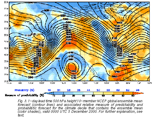), and the climate bin (Fig. 1) where the mean falls is recorded. The number of ensemble members falling in the bin of the ensemble mean is then counted. Just as in the case of the ensemble mode (Fig. 2), a small (large) number of ensemble members falling into the bin of the ensemble mean (supporting members) presumably indicates low (high) predictability. The number of members in that bin is then expressed as a percentile in a frequency distribution of bin counts. This frequency distribution is computed over the preceding 30-day interval¹, and over the Northern Hemisphere (NH) extratropics. 10 (90) % relative predictability at a particular grid point, for example, indicates that 10 (90) % of the grid points had a lower level of predictability during the preceding period over the NH extratropics. These grid points associated with much lower or higher than average predictability were represented by the blue and red success rate curves respectively on Fig. 2 (except that Fig. 2 refers to ensemble mode, and not mean forecasts). These areas of extremely low and high predictability are marked by deep blue and red color shadings on Fig. 3, while intermediate values are marked by intermediate shades of color.

The relative measure of predictability, by construction, is normalized not only by geographical location, season, and lead time but also by the position of the forecast value with respect to the climatological distribution. Note that in the case of a climatologically extreme forecast large spread does not necessarily indicate high forecast uncertainty since the variance of observations and forecasts is generally larger for extreme cases (Toth 1992; Ziehmann 2000). By the use of the equiprobable climate intervals that become wider toward the extremes (see Fig. 1), the relative measure of predictability can be interpreted independent of where the forecast is in the climatological distribution.

c. Probabilistic forecasts

Beyond the various levels of relative predictability, the colors in Fig. 3 are also associated with calibrated probabilistic forecasts for the bin of the ensemble mean. While the relative measure of predictability, by construction, is independent of the lead time and ranges between 0 and 100%, the range of probability values, as suggested by Fig. 2, shrinks and asymptotically tends to the climate probability of 10% when lead time increases. The probability values shown in Fig. 3 are calibrated as described in section 3, using the technique of Zhu et al. (1996) and Toth et al. (1998), based on a preceding 30-day long independent verification data set. Note that the different colors may be associated with more than one bin count. In such cases the calibrated probability value associated with a color is an average of past observed frequency values weighted by the number of points associated with the different bin counts that make up the area with the color in question.

The calibrated probability values reflect forecast uncertainty due not only to initial errors but also to model related uncertainty. This is another advantage of using probabilistic information (instead of ensemble spread) for assessing forecast uncertainty. Note that while initial value related uncertainty is determined in a flow dependent manner based on the ensemble, model related uncertainty, for the lack of its representation in the NCEP ensemble system, is reflected in the calibrated probabilistic forecasts only in a mean sense, averaged over many cases. In other words, the ensemble-based calibrated probabilistic forecasts reflect uncertainties due to both initial and model errors but resolve variations in uncertainty due to initial errors only.

6. Synoptic examples

In this section we present three synoptic examples to demonstrate the dramatic variations in the performance of NWP forecasts that can be objectively identified using an ensemble forecast system. The specific guidance on above or below average forecast uncertainty (section 5) was introduced only recently. Ensemble spread forecasts that have been accessible since 1997, however, can also be used to identify cases with higher or lower than average predictability. All the examples that follow were identified in real time by the authors. The first two examples - one for extremely high, and another for low predictability - will be presented here in terms of mean sea level pressure ensemble spread and probabilistic quantitative precipitation forecasts, while the third will feature the relative measure of predictability for 500 hPa height forecasts.

a. Low uncertainty at long lead time

First we consider a deep low pressure system that developed in the Gulf of Alaska, affecting the US and Canadian west coast around 1200 UTC 6 February 1999. The analyzed mean sea level central pressure of the system had a closed contour of 968 hPa (Fig. 4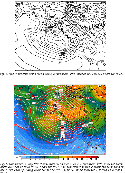), indicating a strongly anomalous flow with a 40 hPa negative anomaly from the long term mean. This cyclone was apparently associated with a very high degree of predictability. It was at 11.5 day lead time when the feature of the anomalous low was first noted in real time using the NCEP ensemble forecasts. And the ensemble mean of the mean sea level pressure forecast did not change much after the initial time of 0000 UTC 27 January (10.5 days lead time), with the deepest closed isobar of the low predicted between 972 and 964 hPa at 9.5 days and shorter lead times.

As an example, in Fig. 5 we present the 9 day NCEP ensemble mean forecast (white contours), along with its associated spread (shades of color). Over large areas of the storm and its environment, including the extreme central low pressure area, the associated ensemble spread (standard deviation of ensemble members around the mean) remained around or below 6 hPa. This is half or less than half of the average ensemble spread computed for the preceding month at this lead time (not shown), indicating well below average forecast uncertainty. The low level of forecast uncertainty is corroborated by the fact that consecutive ensemble mean and spread forecasts valid at the same time (not shown) were very similar. A comparison of the 9 day ensemble mean forecast (Fig. 5) with the verifying analysis (Fig. 4) reveals that the forecasts for this cyclone, as expected from the real time uncertainty estimates, verified very well - the error in the central pressure forecasts was only a few hPa.

Comparing the large scale flow configurations at 12-hour (Fig. 6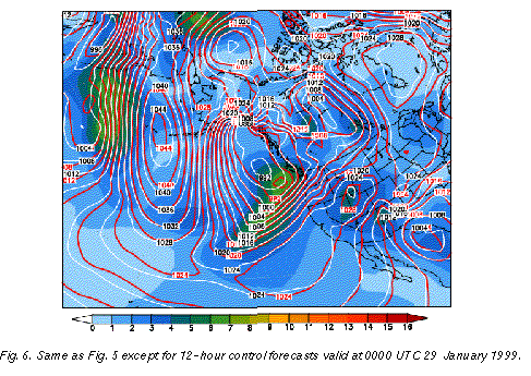) and 9-day (Fig. 5) lead time it is clear that the forecasts were not trivially persisting the observed features present around initial time. Great changes from extremely high to extremely low anomalous pressure conditions were predicted well over large areas, with changes from initial to final state reaching up to 40 hPa over Alaska and nearby areas. Note that the extremely low height values analyzed in Fig. 4 were well predicted by the ensemble mean forecasts (Fig. 5), documenting that the ensemble mean can retain highly anomalous flow patterns as long as these features are highly predictable.

It is interesting to note that analyzed 500 hPa height values near the center of the storm were around 4777 m with a negative anomaly of more than 500 m, falling into the lowest 1% of historical cases based on the NCEP/NCAR reanalysis. At 9-day lead time, 80% (40%) of all ensemble members fell into the lowest 2% (1%) of the climatological distribution, giving a strong indication for the possible occurrence of extreme low values.

The lower than average ensemble spread in Fig. 5 indicates that all members were rather similar. Therefore it is not surprising that the MRF control forecast also verified well. A user with access to only a single control forecast, however, could not have made much use of a control forecast on its own. Given the low levels of average skill at the 9-11 day lead time (less than 20% success rate, see dotted green curve in Fig. 2), forecasts would be issued with a very low level of confidence, that would render them useless for a wide range of users (see, e. g., Fig. 4 of Zhu et al. 2001). Yet with access to information on the widely varying levels of uncertainty, indicated reliably by the ensemble, there are times when extended range weather forecasts with much increased confidence can be made (cf. lightly hatched distribution in Fig. 1, and continuous red curve in Fig. 2).

The above case provides such an example, where confident extended range daily sensible weather forecasts could have been issued based on the ensemble guidance. For example, 12 or more of the 17-member NCEP ensemble forecasts (70-100%) indicated a half inch or more 24-hour accumulated precipitation at 10-day and shorter lead times (Fig. 7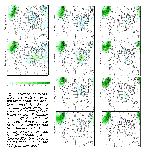) over all areas on the northwest US coast that actually received that much precipitation. Similarly, at 7-day or shorter lead times, the ensemble predicted 70% or higher probabilities for most areas affected by more than an inch of precipitation (Fig. 8b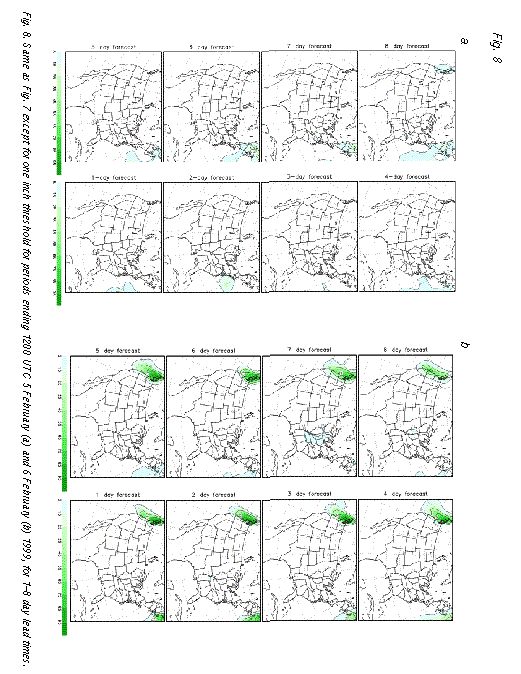). The high degree of predictability in terms of accumulated precipitation may be related to the fact that in this case the precipitation is partly orographically forced.

The time evolution of the weather associated with the storm, as suggested by the unusually low ensemble spread over large areas surrounding the storm, was also well predicted. For example, in contrast to the 70% and higher forecast probability of an inch or more precipitation corresponding to the observed precipitation event around 0000 UTC 6 February, the ensemble correctly gave zero probability at 7-day and shorter lead times for more than an inch of precipitation for the preceding 24-hour period, centered around 0000 UTC 5 February (Fig. 8a).

It is important to note that because the NCEP ensemble does not account for model related uncertainties, small ensemble spread may sometimes be associated with large forecast errors due to model deficiencies. The strong similarity between the NCEP (white contours) and ECMWF (red contours) ensemble mean forecasts, generated by two different models, made the occurence of such errors in this case less likely.

b. High uncertainty at short lead time

The previous example illustrated the potential value of the ensemble approach in identifying weather features associated with low forecast uncertainty, even at long lead times. In this subsection, an example is shown of a case with unusually high forecast uncertainty. Identifying these cases can be especially valuable at shorter lead times where the overall level of forecast skill is relatively high. Interestingly, a prominent example of this kind offers itself in the same forecast studied in Fig. 5, but valid at a very short lead time.

Shown in Fig. 6 is the 12-hour lead time NCEP high resolution control forecast (called "AVN", white contours), valid at 0000 UTC 29 January 1999. A closed low, associated with a cold front extending to the southwest, is seen over the eastern Pacific approaching the west coast of the US. The ensemble spread associated with this system is around 6 hPa. This is the same level of uncertainty found over large areas of the storm studied in the 9-day forecast example of Fig. 5. But while the 6 hPa spread is half or less of the usual spread at 9 days lead time (Fig. 5), it is up to 3 times more than the usual spread at the 12-hour lead time (Fig. 6).

A comparison of the 12-hour NCEP control forecast to that from ECMWF (cf. white and red contours in Fig. 6) confirms the unusually high degree of uncertainty regarding the position of the closed low. The largest differences between the two fields, which reach up to 5 hPa, occur in the area of large ensemble spread. The 5 hPa difference observed between the two control forecasts over the eastern Pacific low pressure system at 12-hour lead time (Fig. 6) is actually above the level of difference present between the two ensemble mean forecasts 8.5 days later, near the center of the Gulf of Alaska storm where the differences are 4 hPa or less (Fig. 5).

Given the high level of average success rate of 12-hour forecasts (65%, see dotted green curve in Fig. 2), a weather forecast based on a single control integration in this case may provide misleading guidance in terms of overconfidence. Information again from the ensemble, in this case based on larger than normal spread, may provide case dependent uncertainty estimates (see the heavily hatched distribution in Fig. 1, and the dashed blue curve in Fig. 2) which are helpful for many applications.

The large differences present within the 12-hour lead time NCEP ensemble, and between the ECMWF and NCEP control forecasts off the northwest US coast in Fig. 6 (around 6 hPa) would certainly be associated with different weather conditions, with the ECMWF forecast, for example, suggesting stronger onshore winds, associated with heavier precipitation. Note that the same northeast Pacific area in the 9-day forecast (Fig. 5) is associated with the same or lesser degree of uncertainty (5-6 hPa ensemble spread and forecast differences).

It is interesting to note that based on the results of Fig. 2, 10-15% of the time a 9-day forecast is expected to be more accurate than 12-hour forecasts on the least predictable 10-15% of cases. It follows that the chances that both a high uncertainty 12-hour forecast and a low uncertainty 9-day forecast would appear on the same day and in the same area is on the order of 1-2%. In other words, in an average year and at any location, 4-6 days are expected when a 9-day forecast can be made with the same or slightly higher certainty than a 12-hour forecast. As a reference, both of these forecasts would exhibit a skill of the level of an average 3-day forecast.

c. Emerging forecast features

The example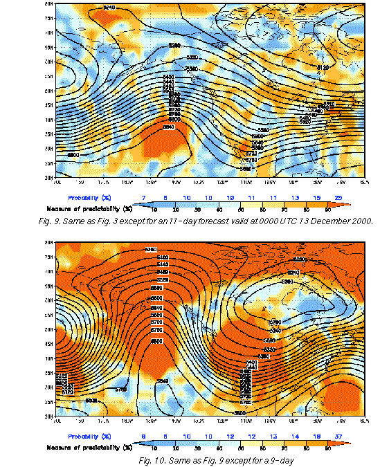 in Fig. 9 displays an 11-day ensemble mean 500 hPa forecast along with the relative measure of predictability and associated probability forecast, valid for 0000 UTC 13 December 2000. The ensemble mean forecast does not have strong anomalies from the climatological mean. Over most of the domain the relative measure of predictability is in the medium to low range, with corresponding probability values close to the 10% climate probability. This suggests, in general, little forecast information in the ensemble, corresponding to a low level of predictability. Fig. 10 shows a 9-day forecast with the same valid time. In contrast to Fig. 9, the ensemble mean forecast is highly anomalous and over large areas the relative measure of predictability is in the 90% range. A number of significant features, among them the deep low pressure system around 170E, the northeast Pacific ridge and the western US trough, are associated with probabilistic forecasts as high as 37%. This indicates, given the long lead time, a relatively high amount of forecast information content with respect to the 10% climatological probability level, that appears just two days after the featureless forecast displayed in Fig. 9.

Interestingly, the 24-hour forecast (Fig. 3) from the same ensemble as shown in Fig. 9 (initiated at 0000 UTC 4 December 2000), indicates a low level of predictability over large areas where the 9-day forecast is highly predictable. In particular, areas in the Gulf of Alaska and over the mid-US show forecast probability levels at the 1-day lead time (<35%) below that marked at the 9-day lead time (37%). Similarly to the examples in Figs. 5 and 6, these are areas where an extended-range forecast contains more information than a short range forecast does. Real time forecast maps like those displayed in Figs. 3-10 can be found at the Environmental Modeling Center's global ensemble web page at: http://sgi62.wwb.noaa.gov:8080/ens/enshome.html.

7. Conclusion and discussions

The analysis of the NCEP global ensemble forecast system in sections 3 and 4 was based on verification results of the ensemble mode and higher resolution control forecasts. Ensemble mode forecasts were stratified according to the value of the ensemble mode, which represents a measure of how tightly or loosely distributed the ensemble members are. The ensemble forecasts were found to possess a substantial amount of case dependent resolution. Therefore they can reliably indicate, at the time weather forecasts are prepared, the large case to case variations in forecast uncertainty. For example, 10-15% of the 1-day forecasts identified as the least and most uncertain by the NCEP ensemble have associated success rates of 92% and 36%; the same numbers for 4 (and 12) day forecasts are 71% and 17% (35% and 11%) respectively.

A further analysis of the results, along with those of other studies (see, e. g., Toth and Kalnay 1995) suggests that on one hand, daily weather prediction for the 6 to 15 days range is possible in cases identified by the ensemble as highly predictable, with the same accuracy and confidence as that of short range forecasts with poorer than average predictability. As Fig. 5 exemplifies, from time to time even extremely anomalous weather patterns can be forecast with high confidence in the extended range. On the other hand, in flow configurations with unusually low predictability, the skill of short range forecasts is expected to be as low as average medium-range, or above average predictability extended range forecasts. We note that the extreme climate categories, as expected from the statistical considerations of van den Dool and Toth (1991), generally exhibit higher forecast success rates than categories near normal. This aspect of the forecast systems have not been evaluated in the present study where success rates were compounded over all climate bins.

The large variations in forecast uncertainty revealed above are a function of (1) the size and distribution of errors in the analysis fields used to initialize NWP forecasts, and (2) the particular evolution of flow patterns from initial to final forecast times. Variations in forecast uncertainty are a direct consequence of the chaotic nature of the atmosphere and are out of the control of the forecasters. Before the advent of ensemble forecasting, forecasters had no or very limited advance knowledge of these changes in forecast uncertainty. With ensemble forecasting, as recent studies have demonstrated, these dramatic changes have become routinely predictable.

Based on the above results NCEP recently introduced, on an experimental basis, geographical displays of probabilistic forecasts for the climate bin in which the ensemble mean falls, out of 10 climatologically equally likely intervals. Areas with above and below average probability values at all lead times are highlighted in red and blue colors respectively (corresponding to the success rates for cases with high and low predictability, like those in Fig. 2) for easy identification of areas with significant deviations from average forecast uncertainty. The new measure offers a bridge between traditional single value (point) forecasts and new, probabilistic type of forecasts.

In the present study ensemble mode forecasts associated with case dependent estimates of uncertainty were evaluated. Ensemble forecasts, however, can also provide full forecast probability distributions, thus further increasing the potential economic value attainable from the use of weather forecasts. Note that such probabilistic forecasts can also be generated based on single control forecasts (Talagrand et al. 1997; Atger 2001). The value of these forecasts, at least theoretically, is limited compared to that attainable through an ensemble of forecasts that can properly account for forecast uncertainty due to initial value and model related errors. In any case the generation and use of probability distributions, instead of single value (or categorical) forecasts requires a conceptual change on the part of the forecaster but this change is necessary for realizing all the benefits an ensemble has to offer.

The performance of NWP forecasts, whether control or ensemble, are negatively affected by the use of imperfect forecast models. The success rates reported in this study, for example, are lower than they would be under ideal conditions, due to simplifications in model formulation. The utility of ensemble forecasts is also limited by shortcomings in the formation of the ensemble. The NCEP ensemble, for example, accounts for forecast uncertainty related only to errors in initial conditions, but not to errors caused by model imperfectness. Therefore the range of foreseeable variations in forecast skill would be wider could we predict the occurrence of flow dependent random or systematic model errors. The results in this and other studies evaluating operational ensemble forecasts naturally reflect all these limiting factors and represent the currently operationally attainable levels of skill. Under these limiting conditions, the ensembles exhibit great value beyond that of single control forecasts, and are ready to be used by forecasters and end users alike. The fact that the system is not perfect and can be improved in the future should not discourage anyone from taking full advantage of what ensemble forecasting can currently offer.

9. Acknowledgements

We are grateful to David Burridge, Director, and the staff of ECMWF, in particular Horst Boettger and John Henessy, for participating in an exchange of ensemble forecasts between ECMWF and NCEP on a research basis. Richard Wobus of GSC provided help with data processing. Steven Tracton, Ed O'lenic, and Peter Manousos of NCEP, John Jacobson (formerly of GSC), and two anonymous reviewers provided helpful comments on earlier versions of the manuscript.

9. References

Anderson, J. L., 1996: A method for producing and evaluating probabilistic forecasts from ensemble model integrations, J. Climate, 9, 1518-1530.

Atger, F., 1999. The skill of ensemble prediction systems. Mon. Wea. Rev., 127, 1941-1953.

Atger, F., 2001: Verification of intense precipitation forecasts from single models and ensemble prediction systems. Nonlinear Processes in Geophysics, under review.

Eckel, F. A., and M. K. Walters, 1998: Calibrated probabilistic quantitative precipitation forecasts based on the MRF ensemble. Wea. Forecasting, 13, 1132-1147.

Ehrendorfer, M., 1997: Predicting the uncertainty of numerical weather forecasts: A review. Meteorologische Zeitschrift, Neue Folge, 6, 147-183.

Hamill, T. M., and S. J. Colucci, 1997: Verification of Eta-RSM short-range ensemble forecasts. Mon. Wea. Rev., 126, 711-724.

Houtekamer, P. L., 1993: Global and local skill forecasts. Mon Wea. Rev., 121, 1834-1846.

Houtekamer, P. L., L. Lefaivre, J. Derome, H. Ritchie, and H. L. Mitchell, 1996: A system simulation approach to ensemble prediction. Mon. Wea. Rev., 124, 1225-1242.

Kalnay, E., and co-authors, 1996: The NMC/NCAR 40-Year Reanalysis Project". Bull. Amer. Meteor. Soc., 77, 437-471.

Kobayashi, C., K. Yoshimatsu, S. Maeda, and K. Takano, 1996: Dynamical one-month forecasting at JMA. Preprints, 11th AMS Conference on Numerical Weather Prediction, Norfolk, VA, 13-14.

Molteni, F., R. Buizza, T. N. Palmer, and T. Petroliagis, 1996: The ECMWF ensemble system: Methodology and validation. Quart. J. Roy. Meteor. Soc., 122, 73-119.

Mylne, K.R., 1999 The use of forecast value calculations for optimal decision making using probability forecasts. Preprints, 17th AMS Conference on Weather Analysis and Forecasting, Denver, CO, 235-239.

National Weather Service (NWS), 1999: Vision 2005. National Weather Service Strategic Plan for Weather, Water, and Climate Services 2000-2005. [Available from U. S. Department of Commerce, National Oceanic and Atmorphseric Administration, NWS, 1315 East West Highway, Silver Spring, MD, 20910-3282.]

Rennick, M. A., 1995: The ensemble forecast system (EFS). Models Department Tech. Note 2-95, 19 pp. [Available from: Models Department, Fleet Numerical Meteorology and Oceanography Center, 7 Grace Hopper Ave., Monterey, CA 93943.]

Richardson, D. S., 2000: Skill and economic value of the ECMWF ensemble prediction system, Quart. J. Roy. Meteor. Soc., 126, 649-668.

Stanski, H. R., L. J. Wilson, and W. R. Burrows, 1989: Survey of common verification methods in meteorology. WMO World Weather Watch Technical Reprot No. 8, WMO/TD. No. 358, 114 pp.

Talagrand, O., R. Vautard, and B. Strauss, 1997: Evaluation of probabilistic prediction systems. Proceedings of ECMWF Workshop on Predictability, 1-25.

Toth, Z., 1992: Quasi-Stationary and transient periods in the Northern Hemisphere circulation series. J Climate, 5, 1235-1247.

_, and E. Kalnay, 1993: Ensemble Forecasting at the N MC: The generation of perturbations. Bull. Amer. Meteorol. Soc., 74, 2317-2330.

_, _, 1995: Ensemble forecasting at NCEP. Proceedings of the ECMWF Seminar on Predictability. Reading, England, 39-60.

_, _, 1997: Ensemble forecasting at NCEP and the breeding method. Mon. Wea. Rev, 125, 3297-3319.

_, Y. Zhu, T. Marchok, S. Tracton, and E. Kalnay, 1998: Verification of the NCEP global ensemble forecasts. Preprints, 12th Conference on Numerical Weather Prediction, Phoenix, AZ, 286-289.

van den Dool, H. M. and Z. Toth, 1991: Why doforecasts for "near normal" often fail? Wea. Forecasting, 6, 76-85.

Whitaker, J. S., and A. F. Loughe, 1998: The relationship between ensemble spread and ensemble mean skill. Mon. Wea. Rev., 126, 3292-3302.

Wilks, D. S., 1995: Statistical methods in the atmospheric sciences. Academic Press, 467 pp.

Zhu, Y., G. lyengar, Z. Toth, M. S. Tracton, and T. Marchok, 1996: Objective evaluation ofthe NCEP global ensemble forecasting system. Preprints, 15th AMS Conference on Weather Analysis and Forecasting, Norfolk, VA, J79-J82.

_, Z. Toth, and R. Wobus, 2001: On the economic value of ensemble based weather forecasts. Bull. Amer. Meteorol. Soc., under review.

Ziehmann, C., 2000: Skill prediction of local weather forecasts based on the ECMWF ensemble. Nonlinear Processes in Geophysics, under review.